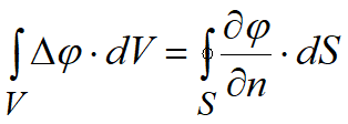
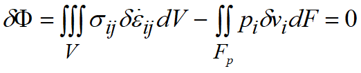
Depending on the type of problem to be solved the defining equation system takes different forms.
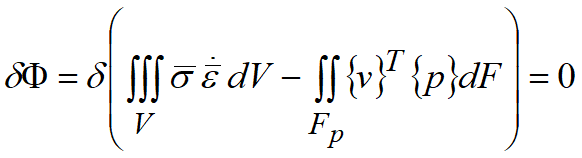
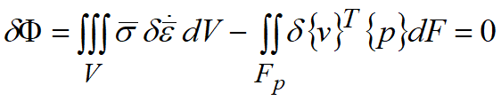
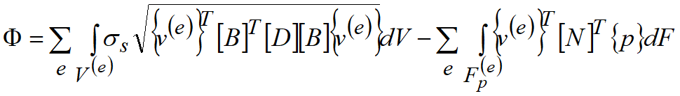
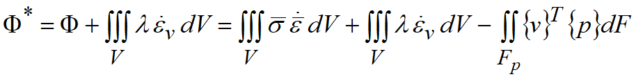
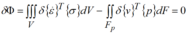
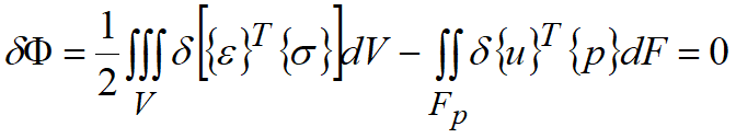
The discrete equations for the problem of rigid-visco-plastic body simulation can be derived by variational formulation that follows from the Markov's functional stationary state
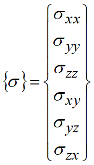
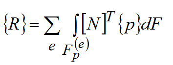
Here:
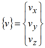
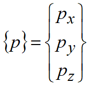
As far as forces and stresses do not vary, then
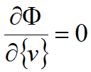
Thus, among all kinematically admissible velocity fields only the true velocity field sets Markov's functional at a minimum value. Necessary condition for functional minimum
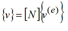
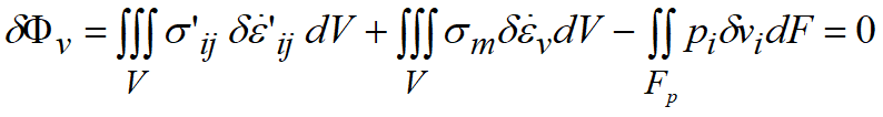
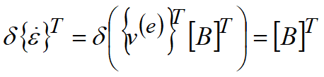
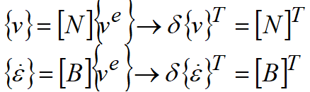
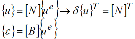
Kinematically admissible velocity field means any field satisfying the essential boundary conditions. At the finite element discretization of deformed body the kinematically-admissible velocity field represents the set of finite elements velocity fields. Velocity field for every finite element in turn depends on shape functions and finite elements nodal velocities:
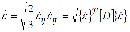
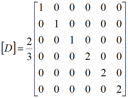
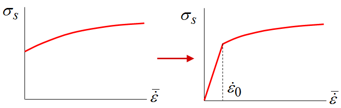
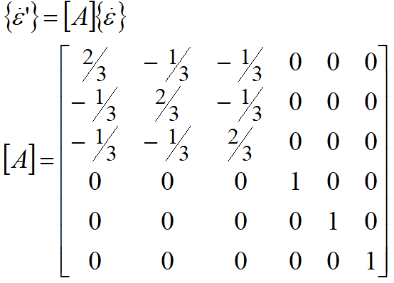
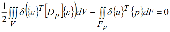
Using von Mises plasticity condition
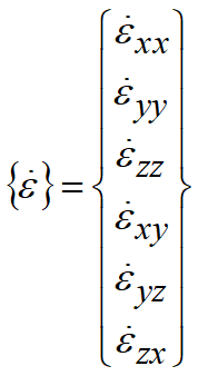
determination of strain rates with respect to finite element approximation of velocity field
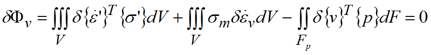
and the determination of the effective strain rate for incompressible body in the matrix form
Here
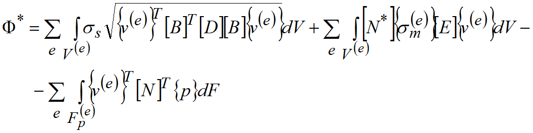
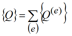
we finally obtain the expression for functional F with respect to the finite-element approximation by summation due to finite elements
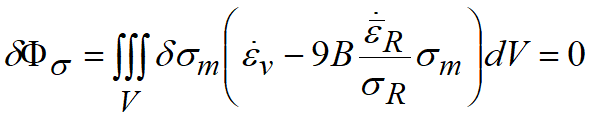
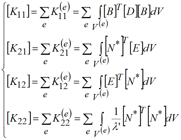
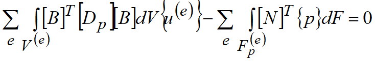
The above formulation in the general case does not satisfy the constrains for velocity field that imposes the volume constancy condition for rigid plastic body that with respect to finite-element approximation can be written as follows:
Here
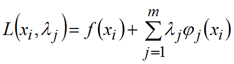
The condition of volume stability imposes additional constraints upon the sought-for velocity field. Therefore, the functional minimum F will be constrained. In order to find this minimum in QForm UKLagrange multiplier method is used. The Lagrange multiplier method is designed for finding the constrained minimum of function taking into account restrictions like equalities. The principle of this method is in the transformation of initial problem of constrained optimization into a task of unconstrained optimization by means of generation of function including constraints. This new function is named as Lagrange function. Let it be necessary to find the minimum of a function that depends on n variables
and also the variables are constrained with m constraints of the type
According to the Lagrange multiplier method the determination of the real function minimum with respect to boundary conditions is equivalent to determination of minimum of a functional
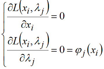
Here l - Lagrange undetermined multipliers. The problem of determining the constrained minimum of function n of variables xi reduces to solution of equation system due to n+m variables xi,λj.
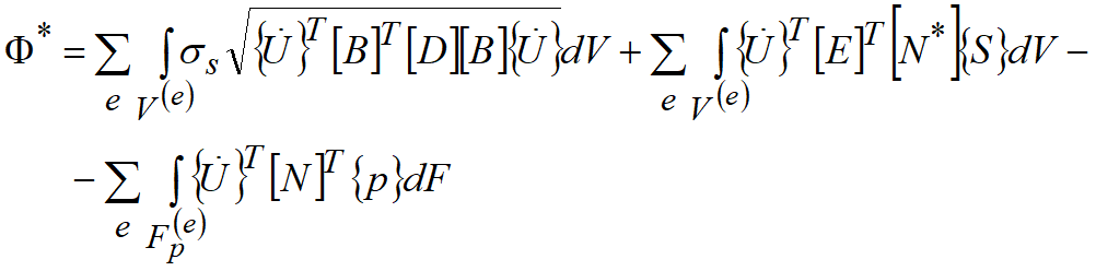
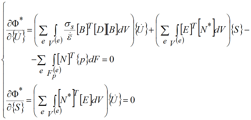
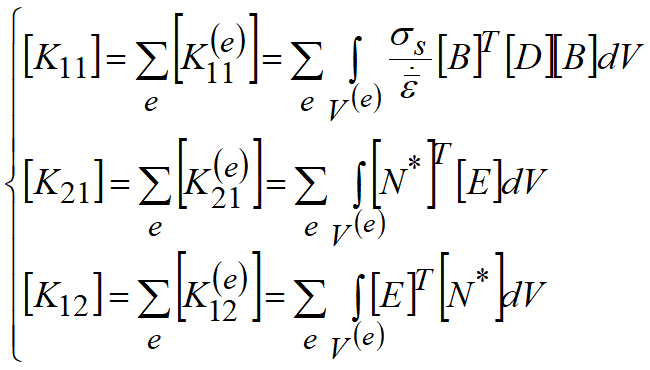
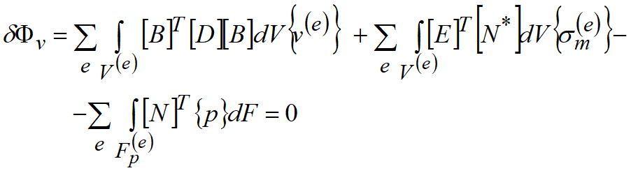
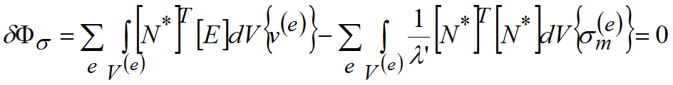
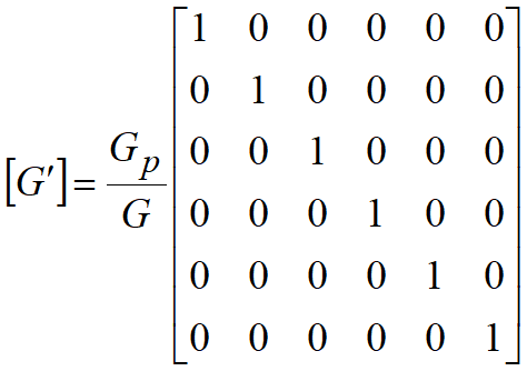
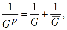
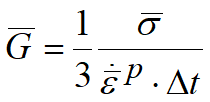
In order to take into account the incompressibility, Markov's functionality is modified by means of introducing the constraints with respect to Lagrange multipliers
Lagrange undetermined multipliers in the reduced functional are the mean stresses
With due regard to finite-element approximation the modified functional takes a form
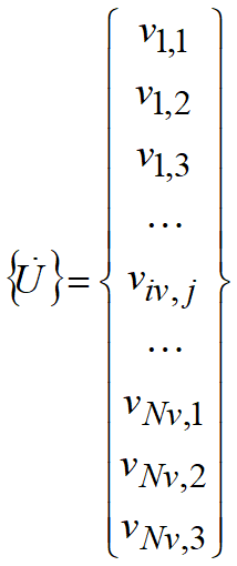
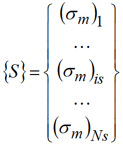
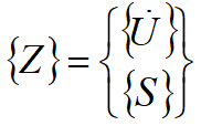
Let's turn to the global coordinate system by introducing the following notations:
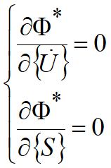
Conditions for functional minimum:
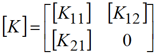
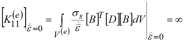
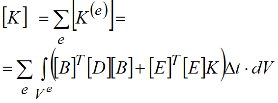
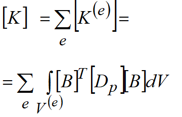
After differentiation we obtain the global equation system.
For transformations the following matrix relations are used
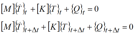
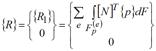
In general terms the global equation system for simulation of strain in visco-plastic body is:
Here
The derived equation is nonlinear, so it requires a multi-step iterative solution.
|


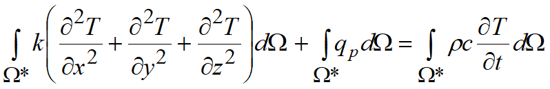
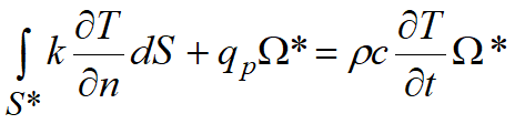
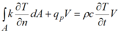
The discrete system of equations for finite element in heat problem is assembled with the use of finite volume method. We use Voronoi cells as finite volumes. On integrating the differential equation of transient heat conduction over volume of a single cell Ω* we obtain
In QForm UK is used in the serial algorithm for a solution to thermo-deformation problems; that is why the integrands for the second and the third integrals are constant. By using the Green formula
in the first integral it is possible to pass on to integration over external area of cell S*. As a result we obtain the heat balance equation for a single cell.
Here n- the normal to the surface of heat transfer. We will explain the principle of generation of equations on the basis of heat balance equation for a cell using the example of a 2D problem.
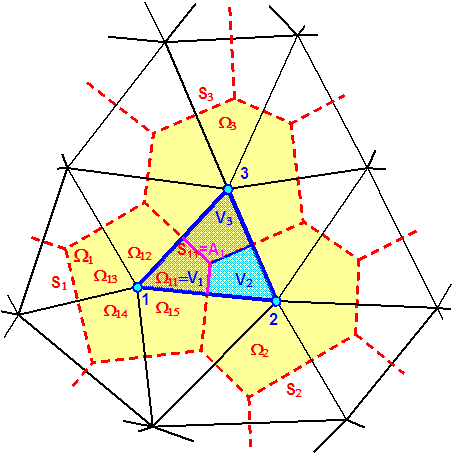
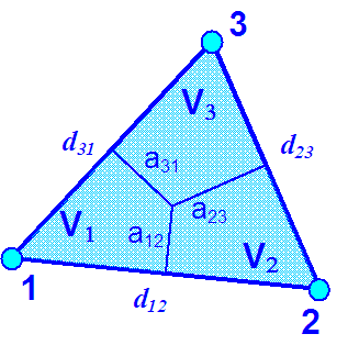
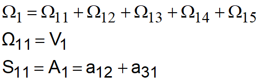
Let's consider a portion of finite element mesh on which the mesh of Voronoi cells is plotted. Every Voronoi cell has a volume Ωi constrained with the surface Si. As far as the mesh of Voronoi cells was plotted on the basis of finite element mesh, then the volume of every Voronoi cell is represented with a sum of volumes that belong to different finite elements. Let's distinguish a finite element based on the nodes 1,2,3. Then the portion of finite volume Ω11 coincides with the portion of finite element V1. Consequently, a portion of external surface S11 represents a polyline A1 consisting of linear elements a12 and a31 perpendicular to the element edges.
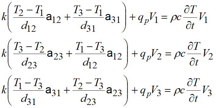
Cell balance equation is also true for any of its components, thus:
As far as the temperature within a cell is considered as constant, and the direction of normal to parts of external surface of Voronoi cells coincide with the direction of vector joining the finite element nodes, then it is true that
Here d is the distance between finite element nodes. Then the heat balance equation for a portion of a finite volume takes a form
Let us write the heat balance equations for the three parts constituting the volume of the finite element
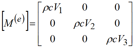
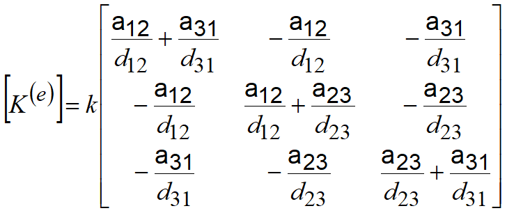
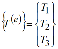
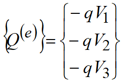
In matrix form, these equations constitute the general system of equations of the finite element. The system of element equations for the three-dimensional problem can be represented in a similar form
For the two-dimensional problem, the components of the matrix element equation, in particular, have the form
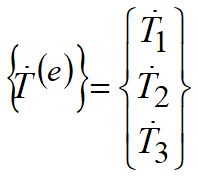
Combining the equations of the elements into a general system of equations taking into account the continuity of heat flows in the nodes, a determining system of equations for solving the problem of non-stationary heat conduction can be obtained
Here
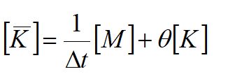
The constitutive system of equations includes both the vector of unknown nodal temperatures and the vector of its time derivatives. The following approximation of the time derivative of temperature is used:
Here
It is assumed that the influence of temperature change on the properties of the body over the integration step can be neglected, then for two close moments of time the constitutive equation of the thermodynamic problem takes the following form
By substituting the values of time derivatives from these equations into the above formula for approximation of derivatives, we obtain the following
After implementing standard discretisation scheme we obtain the global equation system for heat problem due to nodal temperature increments
where
The equation system is linear and does not require an iterative solution. |
||||||||||||||||||||||||||||||||||||||||||

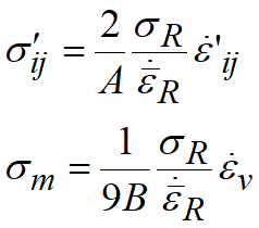
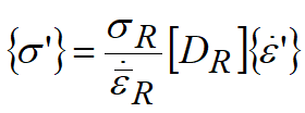
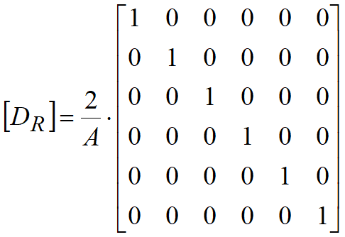
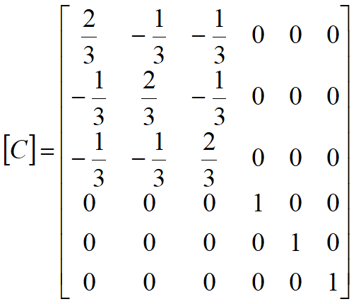
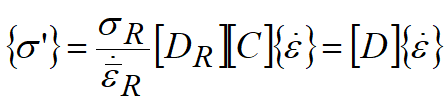
The constitutive equations characterizing the correlations between stressed and strained state of noncompact material have a form
where the first equation characterizes the distortion of workpiece shape (proportionality of stress and strain deviators), and the second one characterizes the change of workpiece volume as a consequence of density change (compressibility equation). Defining equations for problem of noncompact material strain simulation are based on variational equation
Here:
with respect to stress tensor decomposition into spherical tensor and deviator (δij - Kronecker delta)
as well as
we obtain
or in matrix form
Variation form of compressibility equation for non-compact material
The field of velocities and average stresses for every finite element depend on shape functions and nodal values:
Deformation rates are derived from the expressions
In matrix form the correlation between stress and strain deviators (constitutive equations for porous body)
Here
With respect to
where
constitutive equations are reduced to a form
By summing over the finite elements with account of variations
we obtain the final form of variational equations
Let's turn to the global coordinate system by introducing the following notations:
Then in general terms the global equation system for simulation of strain in non-compact (porous) body:
Here
The derived equation is nonlinear, so it requires a multi-step iterative solution. |
 ,
,


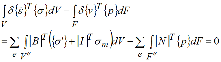
At simulation of thermo-elastic-plastic strain in workpiece during heating and cooling the following relation between stressed state and strained state is used
Here
The defining equations for simulation problem are based on variational equation
Here:
Strain rate tensor can be represented as a sum of deviatoric and spherical components:
Volumetric strain
Therefore
Stress tensor can be represented as a sum of deviatoric and spherical components:
where σm is the average stress Variations with account for finite element approximation
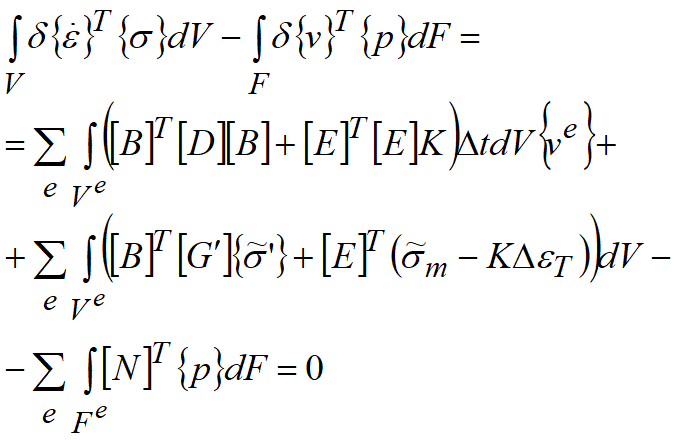
Variational equation takes a form (by summing over finite elements):
The average stress is calculated by means of integration of volumetric strain rate with respect to thermal expansion:
Here
Considering
and
we finallly obtain
Let's turn to the global coordinate system by introducing the following notations:
Then the global equation system for thermo-elastic-plastic strain analysis:
Here
|


Defining equations for the problem of tool elastic strain simulation are based on variational equation:
Here:
Using Hencky's equations matrix form:
Here
we derive variational equation in a form
Given that
and the determination of strains taking into account finite element approximation of displacement field
we finally obtain
Let's turn to the global coordinate system by introducing the following notations:
Then the global system of equations
Here
|


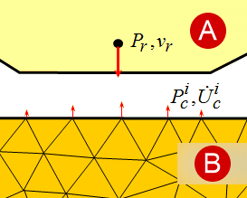
In metal forming processes - the deformation is performed by tools which in turn is driven by processing equipment. The orientation of tool contact surface and the velocity of contact surface points are the boundary conditions for solution of deformation problem. In QForm UK equipment database exist several types of user-available tool drives, which can be united into three grooups: 1. Kinematic equipment (mechanical press, individually driven hydraulic press etc.) - the equipment which operating principle allows assuming that the displacement and the velocity of actuating device are either constant or depend only on time. 2. Energy equipment (hammer, fly press, accumulator power press etc.) - the equipment that the operating principle consists of in the accumulation of potential energy during process pause with its following spending for workpiece deformation work. For this equipment the displacement and the velocity of actuating device depends on spent deformation work. In a general case for this equipment there exists the relation between strain rate and energy.
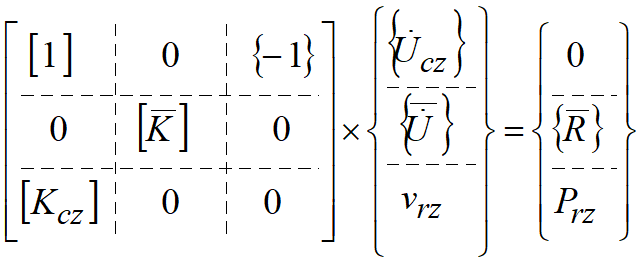
3. Load holder - the tool force applied to a workpiece is constant or depends on time. Tool velocity is determined by the velocities of flow of workpiece material points. If user operates kinematic equipment the modification of the general equation system does not occur. For energy equipment and load holder the "tooling units" are introduced additionally, in which the unknown is the tool speed. As a result, the system is modified. We will consider the principle of equation system modification using a simple example of workpiece and tool contact in the direction of coordinate axis z.
In figure the following notations are agreed:
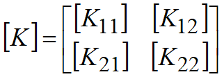
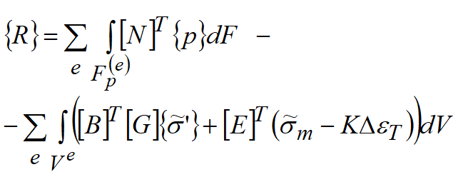
Let us consider the global equation system for workpiece plastic deformation simulation, in which for simplicity we will not account for average stresses as nodal unknowns.
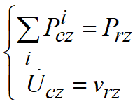
As a consequence of workpiece and tool contact the sum of the contact forces in the nodes should be equal to the force on the instrument, and all the velocities of the contact nodes along the normal to contact surface should be equal to tool speed:
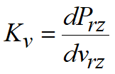
For power equipment the dependence between the speed and the force:
is linearized at the step, then
where
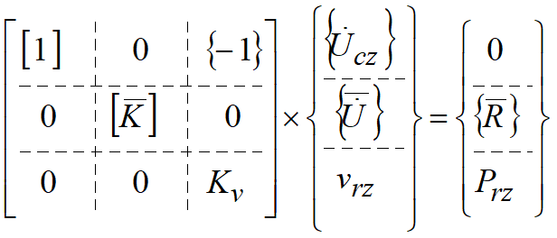
General equation in this case takes a form:
Here
For the case of power pressing the global equation takes a form
where [Kcz] is the stiffness matrix for contact nodes, every element of which represents a sum of system stiffness matrix components corresponding to contact nodes velocities in the direction of normal to workpiece surface (z axis). |