In the general case the governing equations for finite-element method are reduced to systems of nonlinear algebraic equations in the following form
![]()
Here
|
- stiffness matrix that depends on the problem type, analyzed material properties and current geometry |
|
- column matrix (vector) of unknowns in finite element mesh nodes |
|
- column matrix (vector) of reduced external effects to finite element mesh nodes |
The equation is nonlinear. For its solution a multi-step iterative method is used. The whole deformation process is subdivided into a certain number of steps, every one of which corresponds to the system state at a certain instance of time.
![]()
Time step
![]()
is variable and is chosen by the program automatically in compliance with a number of criteria.
At every step a solution is sought for several iterations (i = 1...m). Iteration solution process consists of a sequencing of solutions in the following way
![]()
this sequence converges to exact solution at the step
![]()
with a certain predetermined accuracy.
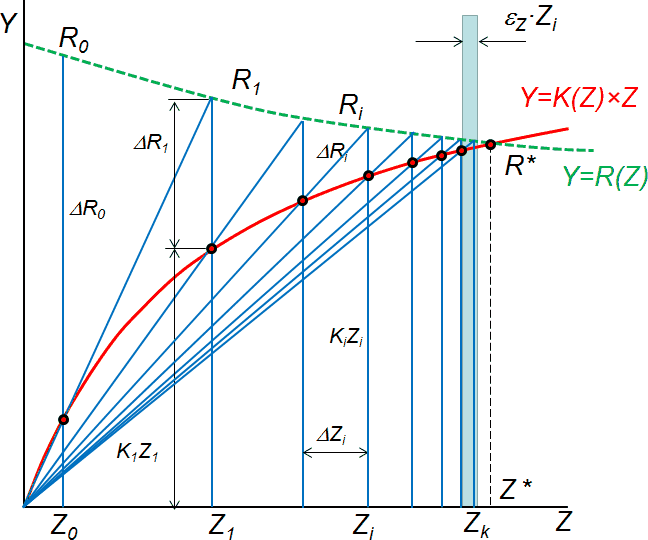
Schematically the step-iterative process can be represented in the following way by the example of nonlinear equation solution
![]()
|
Scheme of step-iterative process of nonlinear equation solution |
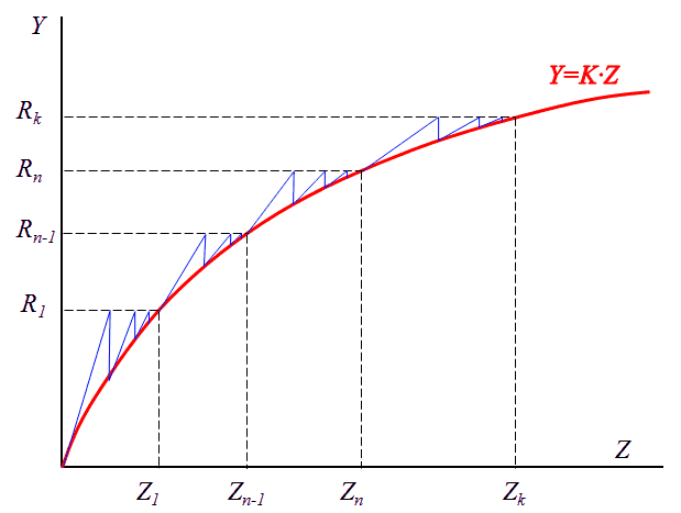
The saw-tooth polyline in figure schematically represents the process of the iterative solution at every step.
Generally the sequence of QForm UK work consists of initial data input, primary generation of finite element mesh and multi-step procedure of solution of deformation and heat problems in the workpiece and tool.
It is necessary to input as initial data the process type (with or without regard to the heat problem), problem type (3D or 2D deformation), workpiece and tool geometry, workpiece parameters, including the parameters of the material rheological model,initial temperature and accumulated degree of deformation, tool parameters, including tool material rheological model, lubricant properties, type and parameters of equipment actuating the tool, boundary conditions, conditions of operation completion etc. See detailed information on the method of initial data input in User's manual.
Multi-step procedure consists in successive solution at every time step of deformation problem for workpiece and tool and of heat problems for workpiece and tool. Deformation problem is nonlinear, so it is resolved with the iterative method.
User has a possibility to choose explicit or implicit method of multi-step procedure organization method.
Simulation step in the program is chosen automatically on the basis of the following criteria: elements degeneration, prediction of time to nodes contact with the tool, the necessity to densify finite element mesh for approximation of geometry and velocity fields, average stress or temperature, requirements of equipment models etc.
User has the possibility to influence the step selection on the Calculation Parameters tab in the Calculation Step section.
The difference between the explicit and implicit methods consists in the way of the determination of finite element mesh nodes location at the simulation step. In QForm UK the nodal unknowns defined in the process of solution are the velocities and average stresses. Thus, the vector of nodal unknowns consists of sub-vectors of nodal velocities and average stresses.
In the explicit method the velocity field is defined for the current system configuration (the coordinates of finite element mesh nodes in the current step). Coordinates of nodes during the iterations remain unchanged. The new step of simulation is defined as proceeding from the obtained velocity field. The system configuration on the next step is defined on the basis of obtained velocity field and the set step according to the formula:
Here
In the implicit method the workpiece shape changes in the course of obtaining the iterative solution in accordance with the velocity field found at the previous iteration by the formula:
Here the average velocity at the step
Thus, the difference between the algorithms of the solution with the explicit and implicit method besides system configuration also consists in the sequence of simulation step determination. The explicit method does not require you to know the simulation step during iterations, and this step can be defined due to the obtained velocity field after the problem is solved; in the implicit method, on the contrary, the value of the simulation step is necessary for the determination of average velocity and is calculated before the iteration starts. The algorithm of explicit at methods:
If the end of the operation has not occurred at the last step, the algorithm is executed again. The algorithm of implicit method:
If the end of the operation has not occurred at the last step, the algorithm is executed again. Heat problem is resolved after the deformation problem, and the solution results are taken into consideration at the next step of the deformation problem simulation. Method selection is available on the tabSimulation parameters in the section General in the branch Integration method. |

General system of equations for deformation problem
is nonlinear. In order to solve it the iterative method of simple iterations is used,which consists of sequencing of solutions (iterations), and this sequence converges to an exact solution with predefined accuracy. At every iteration the initial system of nonlinear equations is reduced to a system of linear algebraic equations in the following way:
Here
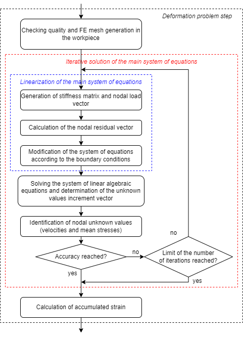
Thus, the algorithm of iterative improvement consists of the following sequence of operations:
In the implicit method after determination of nodal unknowns the improvement of the system configuration is performed. Every iteration consists of several operations, •the first of them is the generation of linear algebraic equations. This is performed in cycle over elements. The results from the previous step can be used at this stage.
•by means of numerical integration the finite element stiffness matrices are determined, and then by means of assembling the system rigidity matrix, the vector of nodal effects and the residual vector is calculated. Consequently:
in order to account for the boundary conditions a modification of the linear algebraic equation system is carried out •The solution for linear algebraic equation system
is derived by the explicit method with respect to the matrix sparsity. As a result the vector is determined of unknowns increments at iteration
•A new iterative improvement of the vector of unknowns is performed
•The condition of iteration completion is checked. The condition for iteration completion is either exceeding the maximum number of iterations or achieving the set accuracy. If the condition is not fulfilled, then the iterative process continues. The last iterative refinement is the solution to the step. •Knowing the nodal velocities at the step we determine the strain rates. By inverting the deformation rates we determine the cumulative strains necessary for the determination of yield stress at the next step.
Schematically the process of iterative improvement can be represented by the example of nonlinear equation solution
in which
The iterations are terminated when the relative increments and residuals became less than the pre-set accuracy.
As far as in QForm UK the vector of nodal unknowns consists of subvectors of different physical nature (velocities and average stresses in finite element nodes)
then the condition of termination of iteration over increments is controlled separately
Here
Euclidean norm of vector. The user has the possibility to change the default values determining the criteria of iteration termination: the minimum norm of velocity increments, the minimum norm of stress increments, the maximum number of iterations. By default the norms of increments due to velocities (main parameter) and average stresses (auxiliary parameter) amount to 3% and 30% respectively of the current norm values for the corresponding quantities. Norms settings control is available on the Simulation parameterstab in General – Iteration. During iterations the contact node can lose its contact with the tool, and at the next iteration it can be regained. This process leads to poor convergence. The user has the possibility to control the process changing the conditions of nodes contact with the tool surface during iterations by means of restricting the number of these separations. By default, the maximum number of separations is equal to 2. If the number of separations during iterations at the step exceeds the preset value, then the motion along the normal to contact surface over contact node is prohibited. Thus, it is "fixed" on the surface and can only slide over it. The criterion of contact separation from the surface is the portion of separation stress calculated as the ratio of normal stress at the contact to the current value of flow stress at the contact surface:
By default, this value is equal to 0.001. |
Global system of equations for heat problem is linear and does not require the iterative solution. Generating the linear algebraic equation system is performed in the cycle over elements. During generation of the linear algebraic equation system by means of integration the heat conductivity and heat capacity matrices are determined, and then by means of assembling the system heat conductivity and heat capacity matrix and the heat flow vector are calculated.
According to the accepted scheme of numerical integration over time the reduced heat conductivity matrix and heat flow vector are determined.
The linearized equation is obtained for determination of nodal temperature increments at this step.
In order to account for the boundary conditions a modification of obtained system is carried out. The solution for linear algebraic equation system is derived by the explicit method with respect to matrix sparsity. As a result the vector of nodal temperature increments at the step is determined.
The new values of temperature are determined by means of summation of obtained temperature increments and temperature values at the current step.
Step of the thermal problem:
It is possible to simulate different heat transfer conditions between workpiece and tool: •No heat exchange •Constant temperature of the tool •Coupled calculation of heat condition of workpiece and tool accounting for lubricant properties •Simple heat transfer of workpiece and tool accounting for lubricant properties. See features for any variant in section "Additional options of simulation" |