In QForm UK a number of additional simulation possibilities that extend the scope of the program and increase the accuracy of simulation in some applications are available. To implement these possibilities it is necessary to set a number of additional parameters.
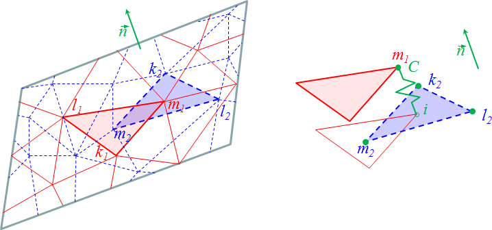
QForm UK provides the possibility of simulating coupled deformation of several bodies. This might be some plastically deformable bodies of the same or different materials (e.g., deformation of the bimetallic workpieces, assembling by means of rivets, etc.) or the tool consisting of several parts assembled together and exposed to small elastic-plastic deformations. Contact surfaces of bodies should not penetrate each other when such processes are simulating, but they can slide relative to each other. Displacements of nodes are used in the capacity of nodal unknowns in the simulation of elastic-plastic deformations of the assembled tools. So the absence of penetration of the contact surfaces is equal to that of the components of the displacements of two contacting bodies that are normal to the contact surface. Since in general the nodes in the finite element mesh in the contacting bodies do not coincide, this requirement cannot be used directly. Special contact element is used for FEM implementation. One node of this element is connected to the node at the contact surface of one body, and the other three are connected to the nodes of the second body constituting a triangle which contains the first node.
At the left of the figure is shown schematically a part of the contact surface without coincident finite element mesh of the first (red solid lines) and the second (blue solid lines) body. The direction of normal is shown with vector n. At the right of this figure the nodes of special contact elements are shown with green dots. For illustrative purposes the contacting surfaces are separated along the normal for a distance comparable with the element size. Let i be the point on the second body surface coinciding with the node m1 on the first body surface. Then
The condition of nodes mutual penetration absence
is fulfilled if the normal force is defined with the relation
is equal to zero. In this case the penalty coefficient C has the dimension of rigidity, and the condition of nodes mutual penetration absence is physically equivalent to the introduction of a contact rigidity between the contact surfaces of two bodies. If the contact rigidity is rather high, then the difference between the normal displacements of contacting surfaces will be negligible. In QForm UK the magnitude of penalty coefficient is chosen as bigger than any diagonal component of stiffness matrix for both bodies in contact.
The displacement of point i can be defined by means of shape function [N] through displacements of the second body nodes comprising a triangle capturing the point. Then:
where
Velocities of nodes are used in the capacity of nodal unknowns in the simulation of plastic deformations of the assembled workpieces. In this case the penalty function providing minimization of penetration along normal to contact surfaces is as follows:
where
Forces in contact element nodes are determined by means of shape functions
where the vector of nodal velocities along normal to contact surface
Penalty coefficient C is determined in the same manner as in the case of the assembled tool: as quantity several times greater than the largest of diagonal coefficients of stiffness matrices for both bodies in contact. Nodal friction forces for assembled tool are defined by Coulomb's law
where μ is the friction coefficient For assembled workpiece the specific friction forces at contact are defined by Siebel's law
where m is the friction factor, k is the maximum shear stress at plastic deformation |
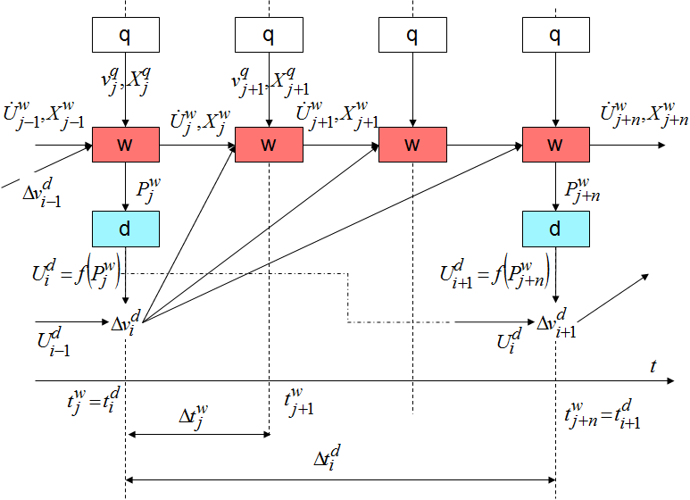
QForm UK gives the user a possibility to select the method of tool deformed state simulation - Coupled tools simulation The user can also choose how to simulate the deformed state of the tool. 1.Stressed state only - Independent simulation of tool and workpiece deformations. 2.Separate - Parallel simulation of tool and workpiece deformations (by default). The interface implements the term "direct deformation". 3.General- Dependent (coupled) simulation of tool and workpiece deformations. Tool deformation in methods above is calculated after determination of workpiece stress-strain state. In the first method the deformed tool shape is ignored in simulation of workpiece deformations, tool contact surface displacement is completely determined with the equipment model. For parts with thin blades (turbine blades etc.), which depth of a cross section is comparable with tool deformation, this solution can cause essential errors. At parallel simulation the tool strain determination is performed at every step of the calculation after simulation of workpiece plastic strains. Contact forces calculated due to plastic strain simulation results and tool displacement as a rigid body determined with equipment model are the initial data for tool strain calculation. After determination of tool deformation the workpiece contact nodes are moved to the tool deformed surface. This method produces a good approximation in the case when tool deformation per step is small. The basic distinctive feature of coupled simulation is in the tool deformed shape simulated at the current step when it is taken into account at the following steps of workpiece deformation simulation. The position of tool contact surface points depends both on the equipment model defining tool displacement as a rigid body and on tool deformation. At simulation of the coupled deformation of plastically deformable workpiece and an elastically deformable tool some problems will occur. The main problems are: 1.Tool geometrical dimensions may essentially exceed the workpiece geometrical dimensions. As a result, adequate simulation of tool deformation may require a number of elements comparable with or exceeding the number of elements in a plastically deformed workpiece. At coupling of elastic and plastically deformed subsystems into a general system of the number of solvable equations, and thus of simulation speed substantially reduces. Here with the plastic part of the system is nonlinear and thus the whole system requires an iterative solution, what also increases the simulation time. 2.At simulation of tool deformation the problem is solved relatively to nodal displacements, and at workpiece deformation simulation - due to nodal velocities. So the divergence of boundary conditions between the workpiece and the tool occurs. For a solution to these problems in QForm UK the following algorithm is used, the solution to workpiece and tool deformation problems are performed separately. Contact forces defined at the current step of problem solution are the external forces for solution of tool deformation problem. Displacement increments for tool deformation step are used for the determination of velocities of points and tool surface shape contacting with the workpiece are the boundary conditions for solution of workpiece deformation problem at the next step. Steps of the solution to the deformation problem in the workpiece and the tool may not coincide. As a rule, step of deformation problem in the workpiece is smaller than the step of deformation problem in the tool. Schematically the algorithm of workpiece and tool coupled deformation is as follows:
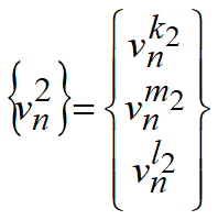
In this figure the following notations are agreed for units of QForm UK: q is the unit for equipment simulation, it defines the tool displacement as a rigid body motion, w - unit for workpiece simulation that determines workpiece stress-strain state, d - unit for tool simulation that determines tool stress-strain state. Let's denote for every workpiece and tool node
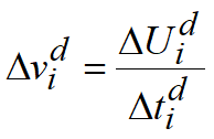
Let us consider the solution algorithm at j-step of plastic problem solution. •The equipment model determines over known time the current velocity and the position in space of the tool as a rigid body. The velocity of the tool contact surface is calculated by means of summation of the velocity of the tool as a rigid body and of the velocity deformation component derived from the solution of deformation problem in the tool at the previous (i-1) step.
•The location of points of tool contact surface are also determined with regard to instrument motion as a rigid body and to velocity deformation component defined as the product of deformation increment of tool velocity
This approach allows accounting for tool deformation at different values of steps over time for elastic task in the workpiece an elastic-plastic task in the tool. Usually the simulation step in the tool is greater than the simulation step in the workpiece:
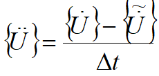
•The derived values for velocities and orientations in space of tool contact surfaces are the boundary conditions at solution of plastic problem. As a result of plastic problem solution the velocities and the locations in space of finite element nodes in the workpiece, as well as in contact nodes are calculated. •Using these forces as external force boundary conditions we can solve the deformation problem in the tool, and as a result tool mesh nodes displacements are obtained
in a moving coordinate system related to the movement of the tool as a rigid unit. •Using the deformational displacements
•are defined the velocities of tool mesh nodes stipulated with deformation at the step of problem solution in the tool:
These velocities are used for determination of velocities and locations of tool contact surface nodes at the steps of simulation of plastic task, in which the tool simulation is not performed. In order to choose the option of coupled simulation of equipment and tool the user has to check the option on the tab Tool parameters. |
At simulation of workpiece plastic deformation the volume change occurs. As a rule the workpiece volume is lost during simulation. The main reason of volume loss is the method of determining nodal locations in the multi-step procedure (e.g. see Kobayashi S., 1989). At multi-step procedure the workpiece new geometry is defined by means of adding the displacements to the previous coordinates. This displacement is calculated by means of multiplication of points velocities obtained as a solution result at the current step (explicit method) or average velocity at the current and the previous steps (implicit method) for the step of simulation over time. Method selection is available on the tabSimulation parameters in the section General in the branch Integration method. The volume loss increases with the growth of deformation and increase of the step over time of multi-step procedure. It should be kept in mind that the volume loss in the implicit method is less than in the explicit method. The volume loss is further caused with a return to the surface of corners that have penetrated inside the contact surface, with cutting of die sharp edges and with the loss of penetrated volume during remeshing, as well as with the number of other reasons. As far as the volume stability law must be observed for rigid-plastic bodies, then in QForm UKby default the option Volume constancy is chosen on the tab in Simulation parameters – General – Workpiece. The method of volume conservation consists in uniform adding of lost volume of to a free surface of deformed workpiece at FE remeshing. This method can cause the workpiece shape distortion that is not stipulated with deformation process. This phenomenon must be taken into account for proper interpretation of obtained results. |
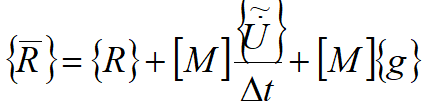
Among possible options of simulation in QForm UK there is the possibility of account for weight (by default) and inertia of the workpiece by choosing Weight (-OZ) on the tabSimulation parameters – General – Consider mass parameters. Workpiece weight is negligible as compared to technological force and causes no influence on deformation process. The main goal of the workpiece weight account is the simulation of the workpiece free positioning in a die under the action of gravity. If due to some reasons the workpiece positioning in the die is to be escaped, then the Weight option in the process parameters is to be unchecked. The account for the workpiece inertia allows analysis of inertial processes at plastic deformation. Problem mathematical formulation (see below) restricts the correct simulation of inertial processes with the cases of simulation with the constant step or with the implicit method. It must be borne in mind that at the first simulation step the loads are not defined. For simplicity let's exclude the average stresses in the nodes from unknowns. Then the defining equation system for plasticity problem solution takes a form:
Here
For complete account for the workpiece inertia this equation should be transformed as follows
where
In QForm UK the nodal acceleration vector is calculated approximately by the formula:
where
With regard to approximate calculation of accelerations the equation system is rearranged as follows
where the reduced stiffness matrix
Reduced vector of nodal loads in this case also accounts for the simulation step over time.
|
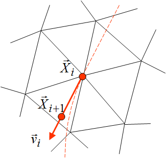
In addition to the effect of volume change in the course of simulation, the multi-step simulation method leads also to a distortion of a motion trajectory of the material points. This is especially noticeable in steady and close to steady processes. Let's consider this problem by using an example of a direct extrusion process. In the course of a steady extrusion process, material points move along trajectories that are close to the trajectory shown in the figure by the dashed line. Consider the motion of a point in the plastic deformation zone for one simulation step. The initial position of the point coincides with one of the nodes of the finite element mesh at the current simulation step.
Using the explicit method, the material point position on the next step of simulation is defined by formula:
where
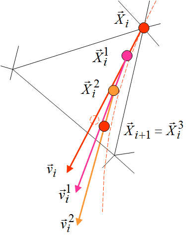
Thus, the point displacement coincides the direction of is velocity vector. The new position of the point will not coincide with its real displacement because the velocity vector in the stationary process in the previous step is tangential. At multi-step displacement the simulation step is divided into several "substeps". The value of the substep:
n - the number of "substeps" Material point position at the sub step is derived from the expression:
where j - the substep number Material point velocity at the substep can be defined directly due to nodal velocities and functions of finite element shape
where
then position of node coinciding the material point at the previous step of simulation will coincide with the position of the material point in the last "substep"
At every substep the position of the point will be positioned in the direction of velocity vector at the substep. The process of multi-step displacement is schematically shown in the figure, from which it follows that the accuracy of tracing the point motion trajectory in this case is substantially increased. For comparison the position of node without a multi-step displacement is shown in the figure with the dashed line
The process of multi-step displacement simulation can be activated by setting the number of substeps in Multistep shift option in Simulation parameters – General – Step shifting. There should not be a large number of steps set in a multi-step displacement. Usually this value should not exceed three sub steps. |
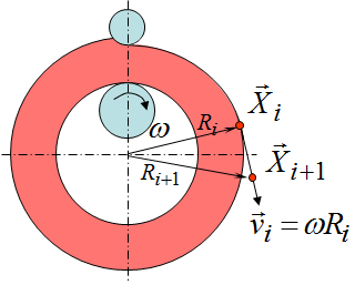
The multi-step simulation leads to changing the shape of the workpiece if the deformed workpiece rotates as a rigid body. Let us now consider as an example of the ring rolling. The deformation zone is located near the rolls. The rest part of the ring rotates as a rigid body.
Let the position of a material point located outside the deformation zone on an external surface of the blank ring of radius Ri from respectively the rotational center at the current simulation step is characterized by the coordinate vector
The position of this point in the next step of simulation for the explicit method will be defined by the equation
Point displacement per simulation step with this method coincides with the direction of its velocity vector at the current step. The new position of the point will not coincide with its real displacement because the velocity vector in the previous step is tangential. It is easy to see that the distance between the point and a rotational centre will increase.
Thus, radius vectors of all material points located outside of the deformation zone will increase from one step to another. The blank "expands" that contradicts a real process. To avoid this effect select the option Rotation in Simulation parameters – General – Step shifting. The distortion of geometry can be prevented by selecting the parameter Rotation to specify rigid body motion. |
The position of the material points during simulation is changing, the initial finite element mesh is distorting and consequently the quality of velocity field and mean stress may go down. Quality of the finite element mesh may be evaluated by the following characteristics: •The size of the finite elements in the area of the maximum gradients of the functions such as stress, temperature, strain, should be minimum, i.e. it is necessary to densify the mesh in these places. •Sizes of adjacent elements should not differ significantly from each other. •Elements with the equal values of the sides (equilateral triangle, regular tetrahedron) are preferable. The penetration of the nodes inside the tool, undercut of the corners caused to necessity of the workpiece remeshing after several steps of simulation. In QForm UK mesh creation is based on a number of parameters, some of which should be set by the user. In most cases it is enough not to change the default values. The Adaptation in QForm UK means the control of the densification of the FE mesh during its generation. The control of mesh generation is based on the "maximum element size" concept. The maximum size of an element means the average length of the element side of the uniform mesh generated automatically with QForm UK. The mesh for any cube will be divided into approximately equal number of elements (near 1200), with side length approximately equal to the maximum size of an element. Adaptation of a finite element mesh to actual geometry of the workpiece is performed in the program automatically. The algorithm is based on a calculation of the maximum distance between sides of the element and a surface of the workpiece with subsequent reduction of element sides until this distance becomes less than a specified number. The following settings of the finite element mesh algorithm process are available to the user: |
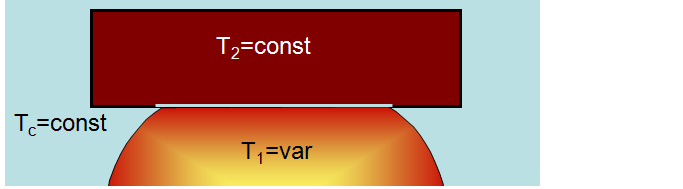
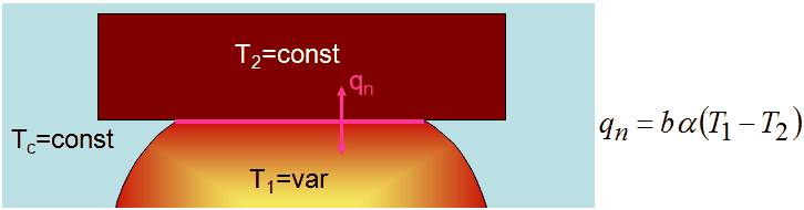
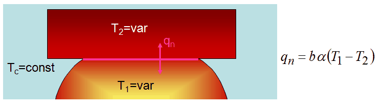
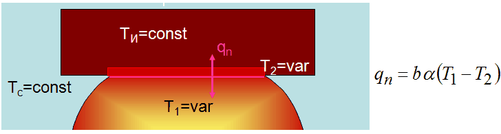
The user is given the opportunity to select the type of heat exchange between the workpiece and the tool on the tab Tool parameters. Depending on the type of heat exchange temperature distribution by workpiece volume will vary. Since resistance to a plastic straining of the metal depends on the workpiece temperature, both strain (flow kinematics) and stress state of the workpiece will vary.
|