Window Graphs opens with a button![]() located on Toolbar. Graphs window can be opened from the context menu called by the right mouse button on the object in Results view window or in the Object tree.
located on Toolbar. Graphs window can be opened from the context menu called by the right mouse button on the object in Results view window or in the Object tree.
To add a graph, click on the button Add graph to the left or Add graph to the right:
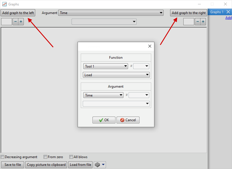
In the window that opens, select Object (tool, trace point or tracking points array), specify Point number (only for tracking points domain) and select Argument and Function, for which the graph is being built.
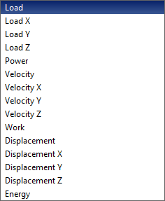
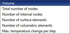
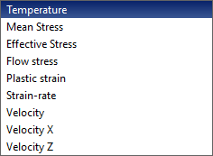
In general, graph plotting is possible for the following functions:
|
|
|
|
|
||
Graphs for the tool |
|
Graphs for workpieces |
Graphs for tracking points |
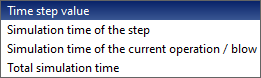
Graphs of simulation parameters |
For plotted graphs, you can change Argument and Value of the graduation:
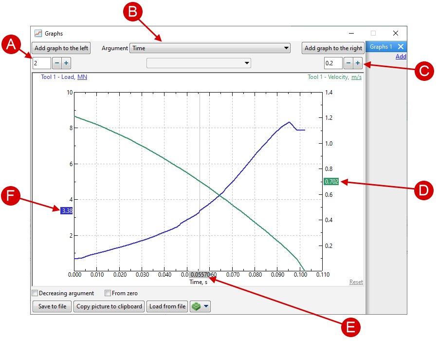
A |
Value of the graduation on the left |
B |
Argument selection |
C |
Value of the graduation on the right |
D |
Function value on the right for the active simulation record |
E |
Argument value for active simulation record |
F |
Function value on the left for the active simulation record |
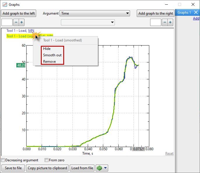
To delete, hide or smooth out the plotted graph, right-click on the graph or the name of the corresponding function and select Remove, Smooth out or Hide:
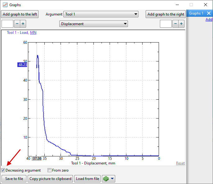
Active feature Decreasing argument plots a graph taking into account the decreasing value of the argument. This feature can be useful, for example, when plotting a function Load from Distance between tools if it is specified as Stop condition:
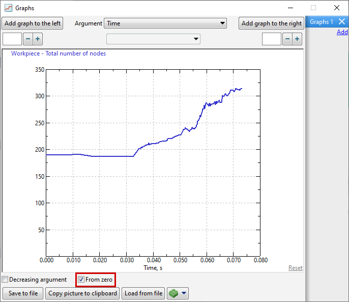
Feature From zero is used when it is necessary to show the origin of the coordinate system, even if the plotted function does not have near zero values.
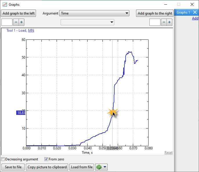
Active simulation record can be switched by clicking on a certain area of a curve:
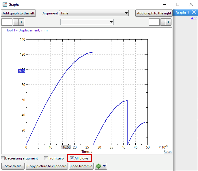
For multi-blow processes, a graph display for all blows is available.
With the commands Add in the right part of the window, you can create additional graph tabs:
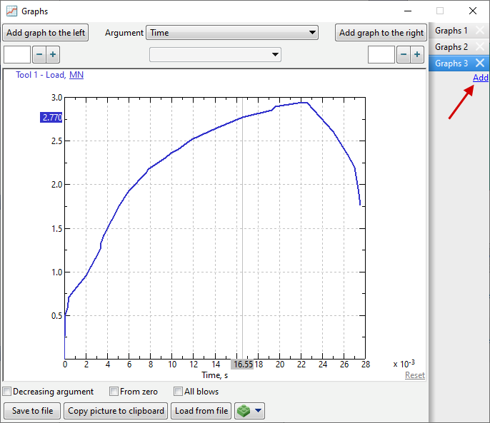
In order to show the graph of the function for a user defined interval on the horizontal axis, it is necessary to select this interval with the mouse:
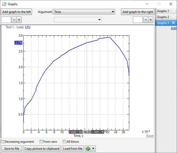
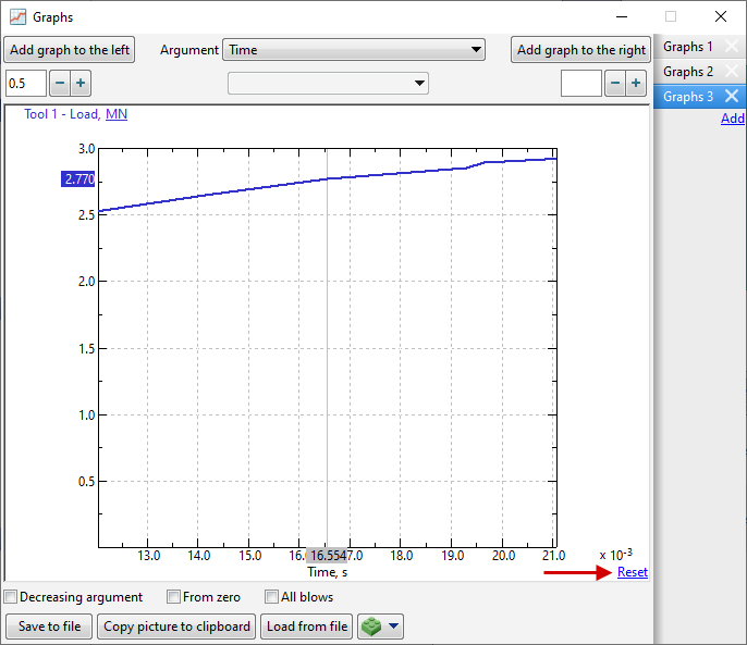
The figure below shows the graph for the selected interval. After selecting an interval, to display all values along the horizontal axis on the graph can be done using the Reset command:
Save to file command at the bottom of the window allows you to export data to *.csv-, *.xls- or *.xlsx-file.
Copy picture to clipboard command saves a bitmap image with plotted graphs to the clipboard.
Load from file command allows you to import data from *.csv-, *.xls- or *.xlsx- file.
In addition, if the Graphs window is open, it is possible to add a graph when Creating animations and images. Graphs window size will match the size of the graph in the animation or image.
|
Information |
||
The graph of the Load function shows the force on the full tool model. In this case, the components Load Z, Load Y, and Load X are calculated only for one calculated sector limited by the planes of symmetry. As a result, the force values shown on the graphs Load and Load Z, Load Y, Load X differ by a factor of n, where n is the number of symmetrical sectors of the full model.
|
|||


See also: