<< Click to Display Table of Contents >> Navigation:  Tutorial > Operation type General forming > Modeling of cyclic heating of the tool

An example of modeling the operation of cyclic heating of the tool with the repetition of the operation of backward extrusion (cold forging) and ejection of the workpiece after extrusion is considered. The simulation consists of two operations: a general forming operation (with the workpiece being ejected in the same operation) and a cyclic heating operation of the tool.

The first forging operation uses the Coupled model of heat transfer between the tools and the workpiece, which is necessary for simulation the cyclic heating of the tool. The Coupled model allows calculation of temperature changes throughout the entire volume of tools, taking into account heat exchange between contacting tools.

In the second operation of the Cyclic tool heating type, only thermal calculation is performed with the accumulation of temperature in the tool for a given number of forging cycles.

The purpose of the simulation is to find out how much the tool will heat up after 50 forging cycles, since in precision cold forging this can affect the dimensions of the resulting forging due to thermal expansion of the tool.

 

 

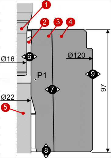
The figure above shows the simulation scheme. 1 - punch, 2 - workpiece, 3 - die, 4 - die holder, 5 - ejector.

Also for this simulation, the following parameters were selected based on the results of experimental studies:

6 - heat transfer between workpiece and the tool

7 - heat transfer between the assembly parts of the tools (taking into account the increase in heat transfer due to tension)

8 - heat transfer with the lower plate or press table (set by the box to reduce the number of finite elements and speed up the simulation)

9 - heat transfer between tools and air.

 

 

Initial data

 

 

1.On the menu File click Open. Specify the path to the project file C:\QForm UK\12.0.1\ geometry\ cyclic_heating \ cyclic_heating.qform . The loaded project will appear on the screen.

2.In the tab Operation check Operation type - General forming, Problem type - 2D axisymmetric and With thermal process, With elastic-plastic deformation.

3.In the tab Workpiece parameters check the material and temperature of the workpiece.

Given material Steels/Carbon steels/C15; 1.0401 cold . Workpiece temperature 28˚С.

4.In the tab Tool parameters it is necessary to check the Drive (1), Temperature and Lubricant (2) for each tool. It is worth noting that in this example Tool 1 - the upper tool, and Tool 2 - ejector. Assembled tool 1 - is a die set with a specified fitting . The material of the tool (3) was selected based on the results of experiments (its thermal conductivity was changed).

 

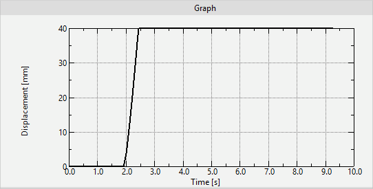
The first operation simulates forging and ejection, so for Tool 1 and Tool 2 drives are specified in the table displacement. The graphs of the tools movement are shown below:

The parameters of friction and heat transfer between the tools were also selected based on the results of experiments (4). The heat transfer coefficient takes into account the tension in Assembled tool 1 . The friction and heat transfer between the ejector and the die are set equal to 0 (5), since their possible contact can be neglected.

So that after simulation of the first operation, the Cyclic tool heating operation can be used , opposite the item Heat transfer to workpiece it must be installed Coupled (6) .

5.In the tab Stop conditions you need to set the process time 8.923 sec, in accordance with the measured cycle duration in the experiment.

6.In the tab Boundary conditions it is necessary to check the environmental conditions for the tools - air 28˚С .

A box is specified for the lower part of the die Environment 1 with modified heat transfer parameters, which determines the heat transfer of the die with the lower plate or table of the press . Click on it and see the environment parameters. Heat transfer coefficient increased to 200 W/m 2 K, and emissivity is set to 0.

7.In the tab Simulation parameters Volume constancy is disabled : the volume of the workpiece is restored only on the free surface of the workpiece in areas with non-zero strain rates, which is not suitable for modeling the reverse extrusion process, in which the proportion of the free surface of the workpiece is small.

The tool mesh parameters are also set as shown in the figure below. These parameter values provide an optimal balance between speed and calculation accuracy:

Click File - Save as and specify a new name and location to save the project on your computer.

8.To start the simulation, click on the button Simulation.

9.After the operation is calculated, open the tab Project , select Operation 1 and click on the button Add operation to process chain .

10.In the tab Operation select Operation type - Cyclic tool heating, Task type - 2D axisymmetric . Click Forward .

11.In the tab Geometry all tools and workpieces are inherited.Therefore press Forward three times before moving tothe Heating parameters tab, because there is nothing additional to be set in the Workpiece Parameters and Tool Parameters tabs.

12.In the Cyclic heating parameters tab set the number of heating cycles in the Maximum number of cycles line.

Install Maximum number of cycles equal to 50 (1) . Activate Save intermediate records - otherwise, only the first and last calculation records will be saved for each stamping cycle. Install Accuracy equal to 0.0001 (2). In this case, all 50 cycles will be guaranteed to be simulated.

In tabs Boundary conditions and Simulation parameters everything remains unchanged. Click OK , save the project and click the button Simulation

13.During the simulation of the operation Cyclic tool heating at each cycle, the heat transfer to the tool calculated in the first operation is repeated. Switching of calculated cycles is carried out by switching of blows on the simulation control panel. The figure below shows the simulation of the 3rd cycle:

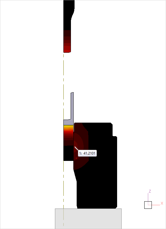
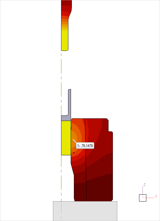
14.After completing the simulation, you can go to multi-window mode and open the first operation in the left window and the second operation (50th cycle) in the right:

15.Tracked point, linesare useful for analyzing temperature change of the tools. The position of the point may correspond, for example, to the location of a thermocouple in an experiment. In this case, it is possible to compare the simulation and the real process. Proceed to step 1 of the first operation. In the tab Traced points, lines select Create point (1), open the drop-down menu (2) and set the coordinates of the point (3): (14.2; 0; 57). Click OK (4).

16.Click Execute tracking for whole chain and wait for the tracing process to complete.

17.In operation Cyclic tool heating right click on Point 1 and in the context menu click Show graphs .

18.Create a temperature-time graph for Point 1 and activate the check-box All blows.

19.Increase the window size Graphs . For comparison with die heating measurements from the experimental study, download the temperature measurement results graph using the button Load from file in the window Graphs . Select the graph experiment_50.xlsx from the directory with the tutorial example.

20.Compare the graphs.

 

See also:

Cyclic tool heating