During the material deformation simulation, the program automatically adapts the mesh of the workpiece based on its own curvature and the mesh density of the contacting tool. This significantly simplifies the simulation process. This section explains how automatic mesh adaptation works in the program and how you can control it.
For most bulk forging simulations, we recommend using the default mesh parameters. This ensures an optimal balance between computational speed and simulation accuracy. In certain cases, depending on the specific task, it is necessary to adjust the finite element mesh parameters of the workpiece and tools before the simulation. It is important to understand that, under certain conditions during the simulation, the workpiece mesh is remeshed, whereas the tool mesh is generated once at the beginning and does not change during the simulation.
Two interrelated concepts are used to describe the finite element mesh of the workpiece or the tool: Adaptation and Element size. The program allows you to control both the adaptation behavior and the element size directly.
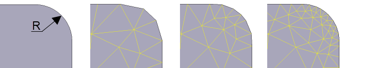
The finite element mesh should approximate the geometry of the tool surfaces and the deformed workpiece with reasonable accuracy. Since the mesh consists of triangular or tetrahedral elements, the element size determines how far the surface represented by these elements may deviate from the parametrically defined input geometry. The smaller the radius of curvature of any surface region, the smaller the elements required to represent that surface with the desired accuracy.
|
The influence of element size on the accuracy of curvature representation |
|
Information |
The principles described below apply to both 2D and 3D simulations |
|
The discussion focuses on the tetrahedral (3D) and triangular (2D) meshes used in most simulations in QForm UK.
Imported 2D objects (from *.dxf or *.crs files) initially have only a surface mesh composed of 1D quadratic elements.
Imported 3D objects (from *.qshape, *.shl, or *.step files) initially have only a surface mesh composed of quadratic triangles.
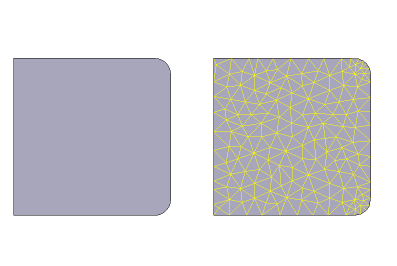
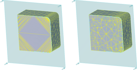
After the simulation starts, the program generates volume meshes for all workpieces and tools. The resulting volume mesh is graded from the surface into the interior up to a certain maximum element size, in accordance with the specified finite element mesh parameters.
|
|
|
2D object before and after creating the volume mesh |
|
Cross-section of a 3D object before and after creating the volume mesh |
To assign volume mesh parameters effectively for the simulation objects, you should first understand the basic characteristics of the FE mesh: mesh adaptation (A), element size (L), the characteristic maximum element size Lmax, propagation of adaptation from the tool surface to the workpiece surface, geometric adaptation driven by the object’s own curvature, and propagation of adaptation from surface nodes into the volume. Only by mastering these concepts the user can meaningfully control the Workpiece mesh and Tool mesh parameters.
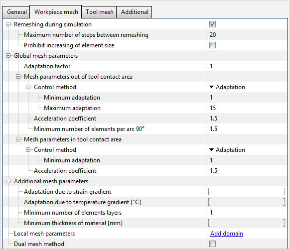
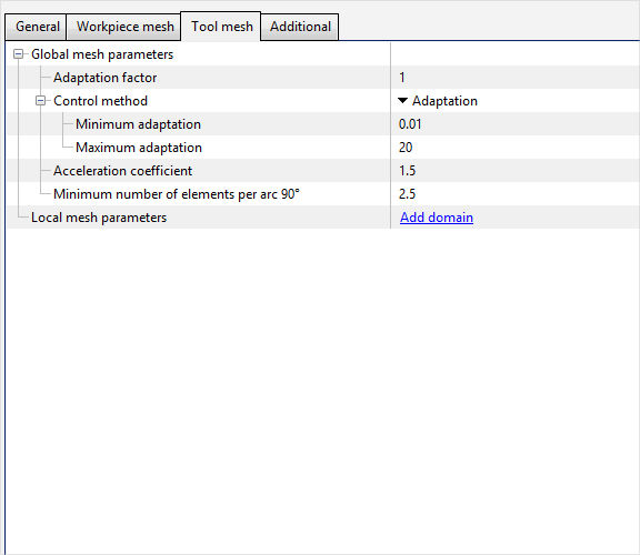
The figure below shows the parameters of the Workpiece mesh and Tool mesh sections:
|
|
|
Workpiece mesh parameters |
|
Tool mesh parameters |
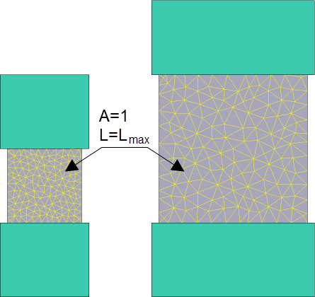
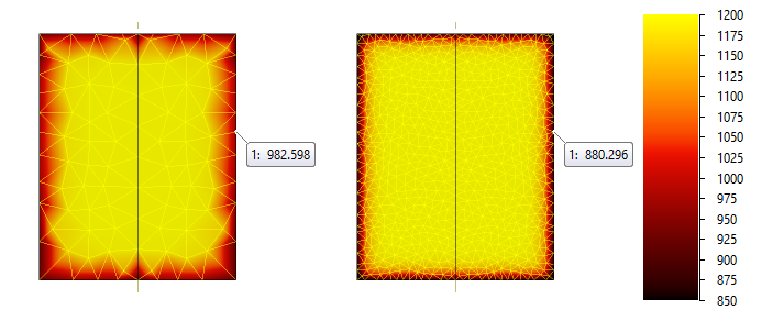
To control the mesh independently of the absolute size of geometric objects, the concept of Adaptation is introduced. Adaptation (A) is a relative quantity computed at mesh nodes and is inversely proportional to the element size (L) associated with those nodes. The higher the Adaptation at a node, the smaller the elements attached to that node, and vice versa. When the simulation starts, the program evaluates a characteristic maximum element size Lmax as a function of the workpiece volume: the larger the workpiece volume, the larger Lmax, and vice versa. At nodes of finite elements whose size equals Lmax, Adaptation = 1. In the figure below, two variants with default mesh parameters are shown. The key difference between them is the workpiece volume:
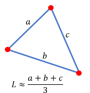
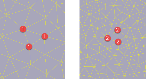
The Element size can be approximately characterized by the average length of the edges connecting its nodes. Each edge connects two nodes that have specific Adaptation values. The greater the Adaptation at a node, the shorter the average edge length around it - and therefore the smaller the elements associated with that node.
Adaptation at a node is defined as the ratio of the maximum characteristic element size Lmax to the average edge length around that node, or, simplistically, to the average size of the elements belonging to that node: A = Lmax / L The element size is inversely proportional to the adaptation value: L = Lmax / A Thus, if Adaptation = 1 at a node, the average size of the elements attached to that node tends toward Lmax.
|
||||||||||||
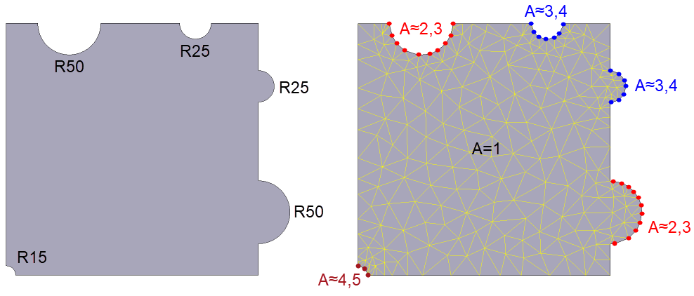
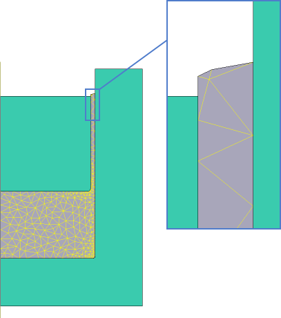
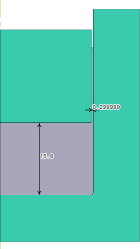
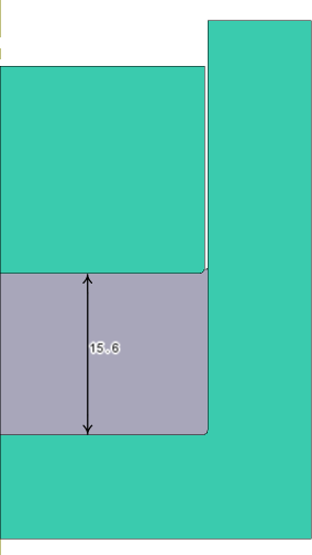
The process of automatic volumetric mesh creation can be divided into two stages: 1. Applying geometric Adaptation to the body surface. 2. Acceleration of Adaptation from the surface throughout the entire volume of the body. The principle of geometric adaptation driven by an object’s own surface curvature applies equally to both the Workpiece mesh and the Tool mesh. The only distinction is that the workpiece surface curvature may evolve during the simulation and therefore influences the Workpiece mesh, whereas the Tool mesh is generated once and remains unchanged throughout the simulation. Element sizes for representing curved surface regions are assigned automatically so that their deviation from the represented surface does not exceed a specified tolerance, which in turn depends on the workpiece volume. On the cross-section shown below on the left, there are straight segments and five fillets. On the left, the fillet radii are indicated; on the right, a generated mesh with default simulation parameters is shown.
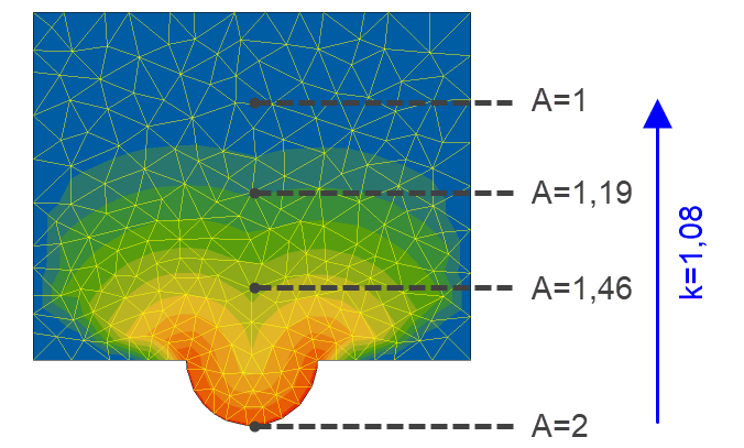
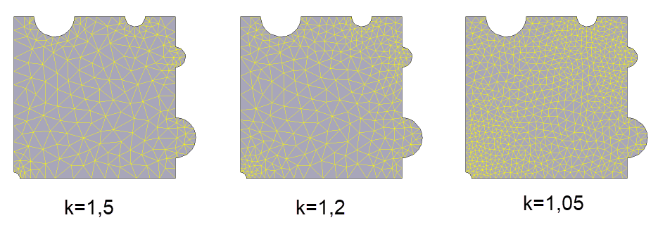
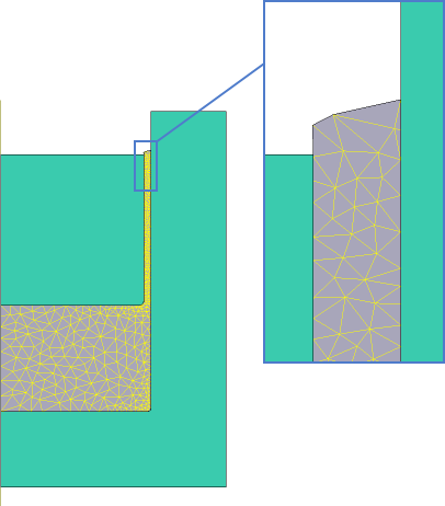
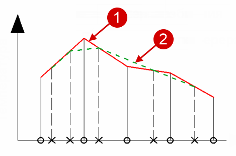
Moving away from the curved surface region into the volume, elements coarsen up to the maximum element size specified in the Simulation parameters. Coarsening occurs gradually with an acceleration coefficient k, defined in the mesh parameters. With increasing distance from the curved surface, the adaptation value of each subsequent element layer is reduced by a factor of k, until the minimum adaptation value is reached, which by default is 1 and corresponds to the element size Lmax. The principle of accelerating the workpiece mesh from its own curvature is shown in the figure below:
Thus, the smaller the acceleration coefficient k, the slower the enlargement of elements as they move away from the source of adaptation. Thus k ≥ 1. When k=1, the size of all elements will approximately match that of the smallest element on the surface of the object.
|
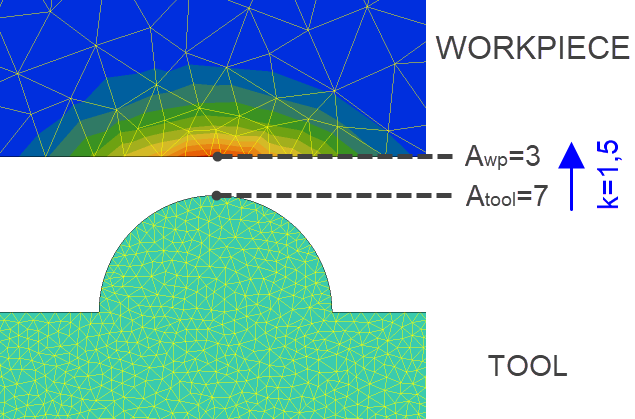
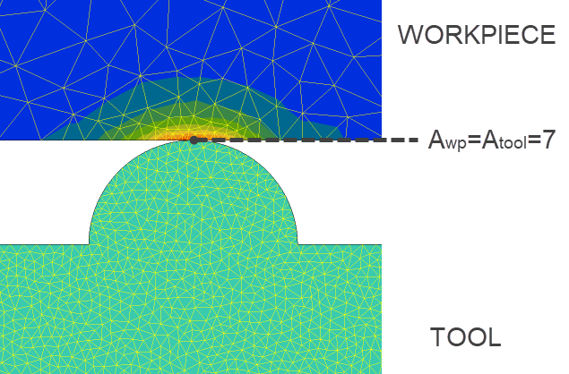
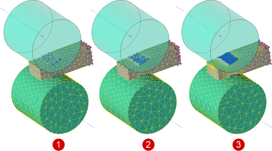
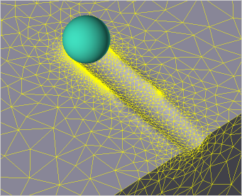
Applying adaptation from the tool to the workpiece can be divided into two stages: 1. When the tool is not in contact with the workpiece, adaptation from the tool surface is accelerated to the surface nodes of the workpiece mesh with an acceleration coefficient of k=1.5. This is a system constant that cannot be changed. The figure below shows the tool positioned at a certain distance from the workpiece. The Tool mesh in this example has been intentionally refined using the mesh parameters to make the propagation of adaptation from the tool to the workpiece clearly visible:
2. As the tool approaches the workpiece, the adaptation applied to the workpiece surface increases. Upon contact, the contact nodes of the Workpiece mesh inherit the Adaptation of the Tool’s contact surface. In other words, at contact the Tool and Workpiece have the same mesh density - but only if the Workpiece mesh was coarser prior to contact:
|
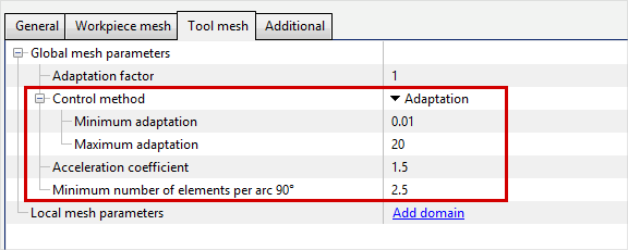
When configuring the Workpiece mesh and the Tool mesh, you should first focus on the Tool mesh parameters. The generated volume mesh must approximate the tool’s forming surface with sufficient accuracy. In many cases, it is enough to tune only the Tool mesh parameters, because the Adaptation of the tool’s forming surface is propagated to the contact nodes of the Workpiece. To configure the Tool mesh correctly, it is sufficient to understand how four fundamental parameters jointly affect the mesh: •Minimum adaptation •Maximum adaptation •Acceleration coefficient •Minimum number of elements per arc 90°
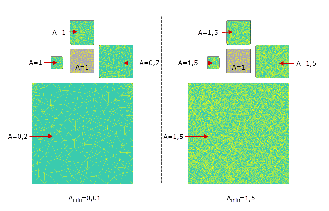
In the figure below, an example is shown with a workpiece and four tools. One tool is smaller than the workpiece; the second has the same volume as the workpiece; the third and fourth tools are larger than the workpiece. As noted above, the characteristic maximum element size Lmax (for which Adaptation A = 1) is computed based on the workpiece volume. By default, the Tool Minimum adaptation is 0.01. This is set so that the tool element size can grade (coarsen) away from curved surfaces into the interior to values larger than Lmax. Tools are usually larger than the workpiece, so there is no point overloading the simulation with an excessively dense mesh inside the tool. In practice, the target A=0.01 is rarely reached during grading; however, this setting allows the tool elements to grow as much as possible in the interior. If the tool volume is equal to or smaller than the workpiece volume, then with the default settings the Adaptation at tool nodes cannot drop below A=1. The larger the tool volume relative to the workpiece, the larger the maximum element size the Tool mesh can grade up to when Minimum adaptation is set significantly below 1. If, for example, you set Minimum adaptation = 1.5 in the Tool mesh parameters, then for all tools the maximum element size reached by grading will correspond to Adaptation = 1.5.
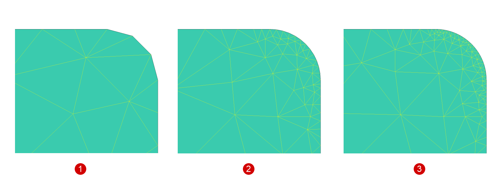
Maximum adaptation is a very important parameter. It limits the minimum element size of the generated volume mesh. If the object geometry contains curved regions that require a higher adaptation than the specified Maximum adaptation, those regions will be represented coarser than necessary. Acceleration coefficient. The principle of this parameter was detailed above. The default value is usually suitable. In some cases, when you need to slow down coarsening into the interior, you can decrease this value. Minimum number of elements per arc 90°. Defines the minimum number of elements that must be guaranteed on a curvature segment of 90°. By default, the tool uses 2.5. This means any 90° arc will be described by at least 2.5 elements, and a 180° arc by 5 elements. Note that the specified Maximum adaptation constrains the effect of this parameter.
|
Non-contact nodes of the Workpiece mesh are nodes where there is no contact with the Tool. In the figure below, the contact nodes of the Workpiece mesh are marked with blue and pink points. All other nodes are non-contact. The Tool was intentionally given a denser mesh, and it is clearly visible that on the contact surface the Workpiece inherits the Adaptation from the Tool surface - the elements on the contact area of the Workpiece surface are significantly smaller than those in the interior and on the non-contact area of its surface:
When the tool is not in contact with the workpiece, all nodes of the workpiece in this example become non-contact, and the Mesh parameters out of tool contact area are applied to them - including to nodes that were previously in contact. In the figure below you can clearly see that the elements on the area of the surface that was previously in contact coarsen after the tool is withdrawn:
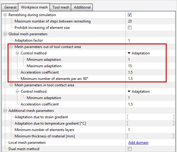
The Adaptation at non-contact nodes of the workpiece is determined by the parameters set in the Mesh parameters out of tool contact area block:
|
||||
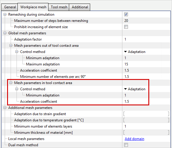
In some cases - when the Tool’s contact surface is meshed coarser than the Workpiece’s contact surface - you need to refine the Workpiece mesh in the contact area (e.g., in longitudinal rolling or open die forging). Using Minimum adaptation (default 1) and Acceleration coefficient (default 1.5) in the Mesh parameters in tool contact area block, you can assign a finer Workpiece mesh directly in the contact zone and specify how the mesh grades into the workpiece volume starting from the contact nodes:
|
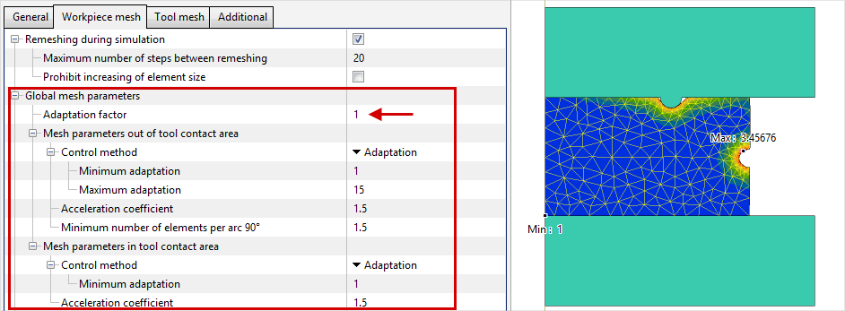
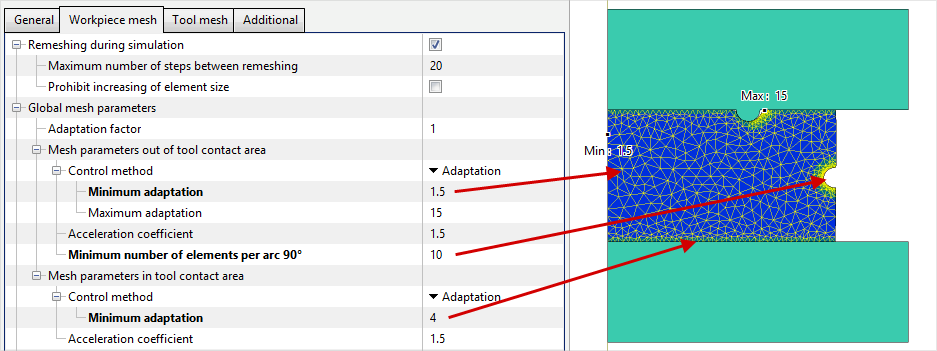
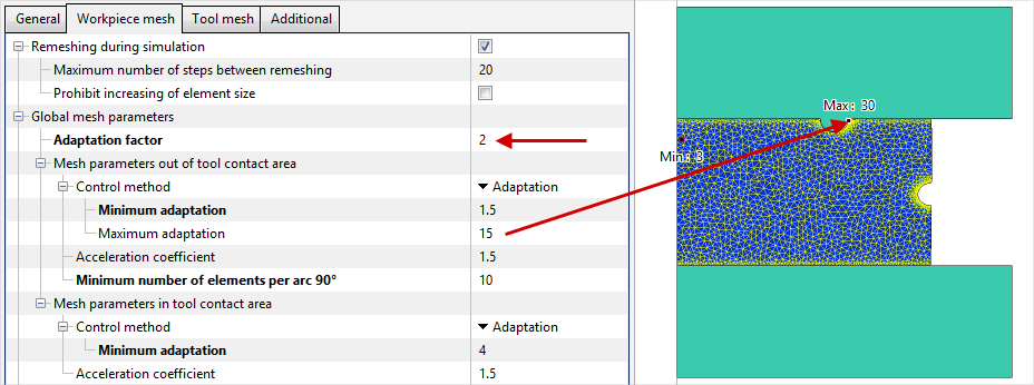
The most intuitive and widely used mesh-control parameter is the Adaptation factor. The Adaptation values computed at all mesh nodes are additionally multiplied by Adaptation factor. In other words, the Adaptation factor scales the finite element mesh obtained with all curvature-driven effects and other mesh parameters, including Minimum adaptation and Maximum adaptation. An Adaptation factor > 1 refines the Workpiece or Tool mesh throughout the region where it is applied (globally or locally). An Adaptation factor < 1 makes the mesh coarser. The figures below illustrate how the Adaptation factor works in combination with other mesh parameters.
The Adaptation factor is useful, for example, when you need to perform a quick preliminary simulation. The figure below illustrates this case.
|
||||||||||||||||
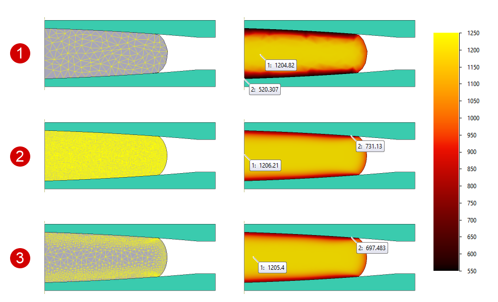
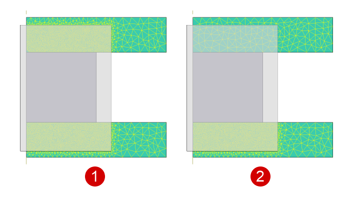
For a more accurate solution of the thermal task in the workpiece, the program can automatically refine the mesh in regions with steep temperature gradients. When this parameter is enabled, the workpiece mesh is constrained so that within any element the difference between the maximum and minimum temperature does not exceed the specified limit. As the figure below shows, achieving an accurate thermal solution does not require a fine mesh throughout the entire workpiece volume; Adaptation due to temperature gradient allows you to obtain nearly the same result:
The mesh adaptation achieved by considering Adaptation due to temperature gradient cannot exceed 10. |
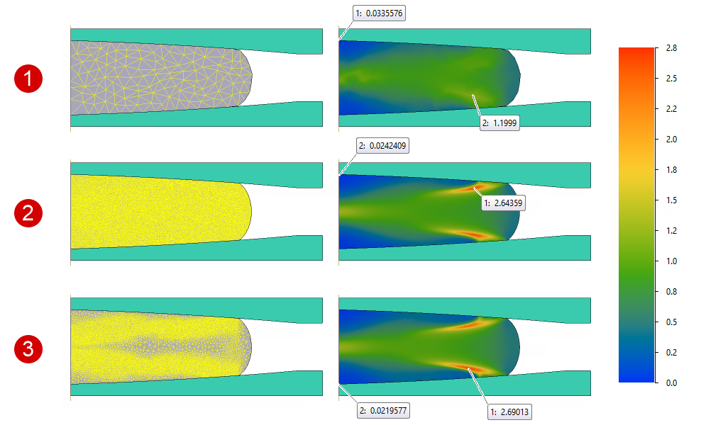
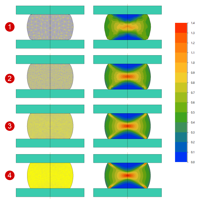
To achieve a more accurate description of the accumulated strain distribution in the workpiece, the program can automatically densify the mesh in the most deformed regions of the workpiece. When this parameter is used, the workpiece mesh is generated in such a way that the difference between the maximum and minimum values of accumulated strain within any element does not exceed the specified value. As the figure below shows, obtaining an accurate distribution of the accumulated plastic strain field does not require a fine mesh throughout the entire workpiece volume; Adaptation due to strain gradient allows you to achieve nearly the same result:
The mesh adaptation achieved by considering Adaptation due to strain gradient cannot exceed 10. |
In some processes, the material of deformable workpiece can penetrate into tight clearances between the tools. To ensure the required number of elements through the thickness of the material flowing into the gap, use the Minimum number of elements layers parameter.
|
In the simulation of some processes, such as the forging of copper alloy fittings, the material may begin to flow into very narrow clearances between the tools. As a result, the workpiece ends up with a very large number of elements, which slows down the simulation. The Minimum thickness of material parameter allows the program, during the simulation, to remove elements in regions where the workpiece thickness is less than the specified value.
|
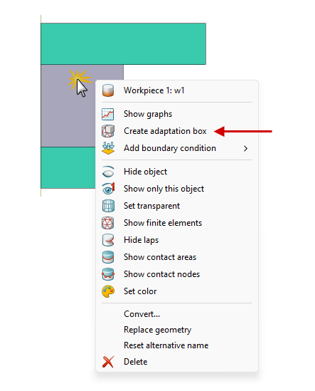
In some cases, you need to assign specific mesh properties only to local regions of the workpiece or tool. For this purpose, you can create so-called boxes in the mesh parameters - volumes with a defined shape and size - and, using positioning, place them in the required areas of the workpiece or tool. There are two ways to add a local mesh-parameter region to the simulation: •right-click on the desired object in the results view window and select the Create adaptation box command from the menu
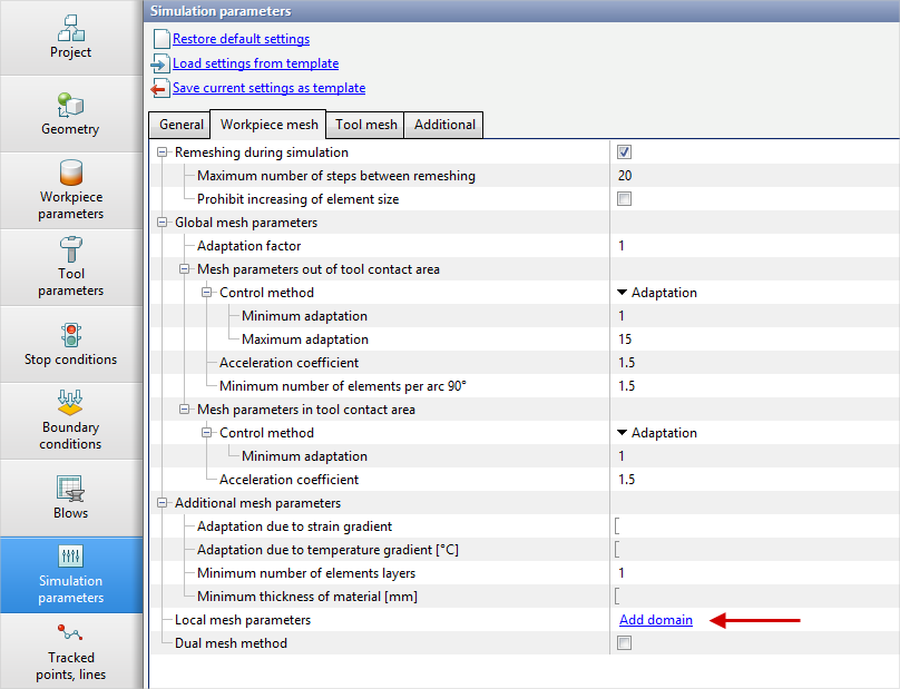
•In the Workpiece mesh or Tool mesh sections of the Simulation parameters tab, execute the Add domain command in the Local mesh parameters row
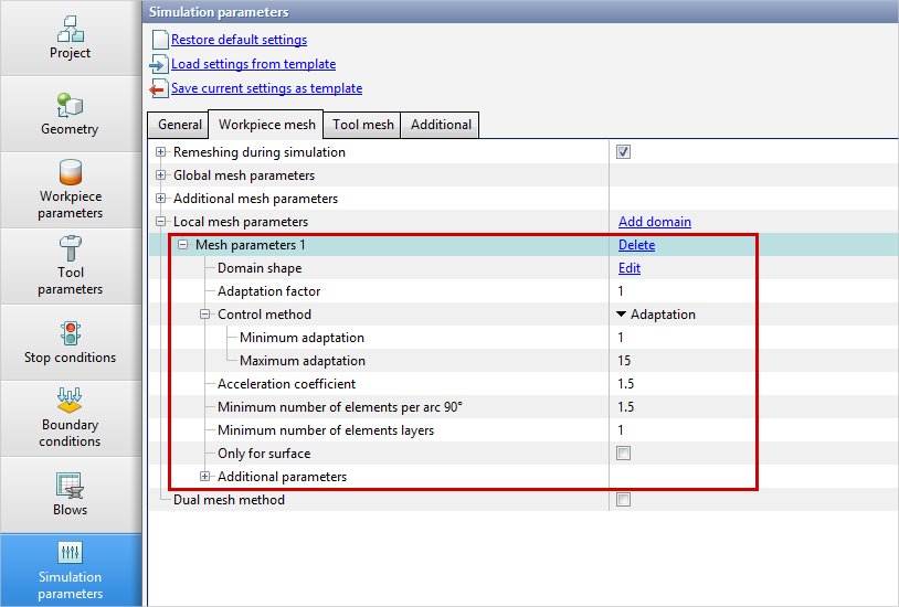
As a result, the additional mesh parameters block for the created local area will appear in the list of workpiece or tool mesh parameters:
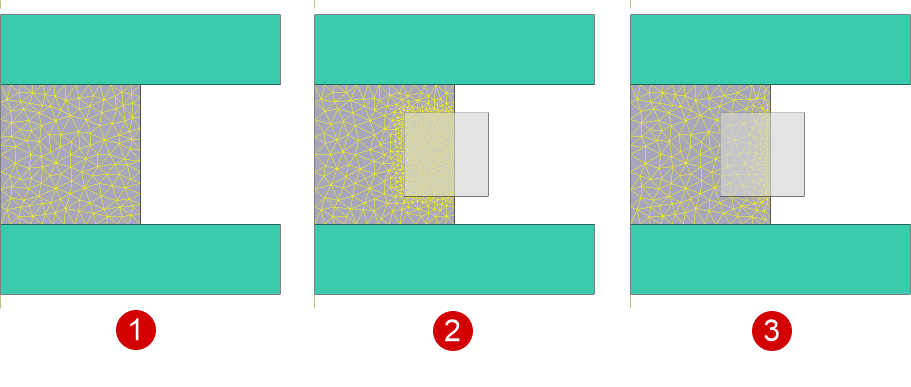
In 2D simulations, a local mesh parameter area can have the shape of a rectangle, a circle, or an arbitrary contour imported from a *.dxf file. In 3D simulations, a local mesh parameter area can have the shape of a cuboid, a cylinder, a cone, a sphere, or an arbitrary body imported from a *.step file. See also: By default, a local mesh-parameter region applies to all mesh nodes of the object that fall within it. If you enable Only for surface, the region applies only to the object’s surface mesh nodes located inside that region.
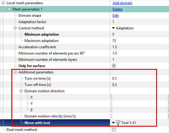
In the Additional parameters block of the Workpiece mesh section, you can set the velocity and direction of the domain motion, attach the domain to a specific tool, and specify its turn-on and turn-off times. If the simulation involves several workpieces, you can select the specific workpiece to which this area should be applied.
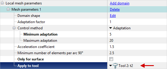
In the Additional parameters block of the Tool mesh section, you can select the tool to which the created domain should be applied.
Previously created local mesh-parameter regions can be deleted or edited using the corresponding commands in the Simulation parameters tab, or via the right-click context menu in the results view window. |
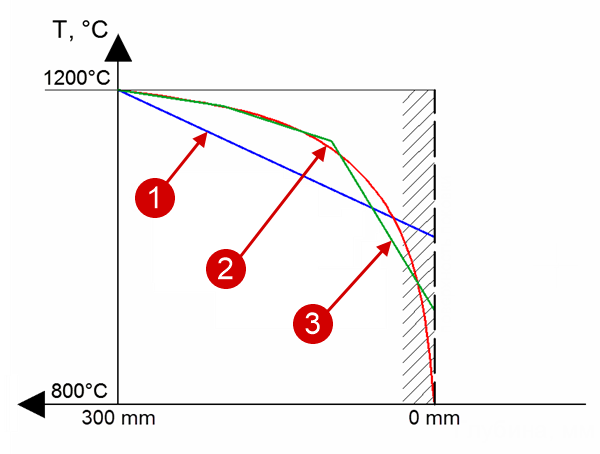
Let us examine how the element size affects the accuracy of temperature calculation on the free surface of a cylindrical workpiece during air cooling. The thermal problem is solved in the software using the finite volume method based on the applied finite element mesh. The temperature distribution is a linear function in the element, with the temperature values at the nodes calculated based on the energy balance. The figure below shows that a threefold reduction of the element size significantly brings the values at the nodes of the piecewise linear function closer to the analytical dependence. As seen, when a coarse mesh is used, the surface temperature during cooling is significantly higher than the analytical relation predicts. This is due to enforcing the energy balance: the heat removed from the surface can be taken only from the entire element:
Another FE-mesh property that introduces additional error is remeshing, which occurs due to automatic adaptation in the tool contact area or on the workpiece free surface, as well as when deformed elements undergo element degradation. After remeshing, the approximated distribution of the computed field prior to remeshing is mapped onto the new mesh, and the transferred values are assigned to the new nodes. The new distribution over the entire volume is then constructed as a piecewise-linear function of these transferred values - schematically illustrated for a one-dimensional problem in the figure below:
The figure below presents a simple example of simulating the upsetting of a large billet with a diameter of 2000 mm and an initial height of 2500 mm down to 1500 mm. During upsetting, the air cooling time was set to 200 s, and the upsetting process time to 100 s.
There is always an optimum finite element mesh density, beyond which further refinement results in only a marginal improvement in simulation accuracy. Therefore, in all simulations, it is recommended to follow a balanced approach - a "golden mean" - when it comes to mesh density. Keep in mind that, in addition to FE-mesh parameters, many other factors can affect the numerical simulation error. Increasing the finite element mesh density improves the accuracy of the calculated fields, but also leads to longer computation times. Depending on the type of the simulated process and the dimensions of the deformable body, optimal finite element mesh parameters can be selected for the particular task.
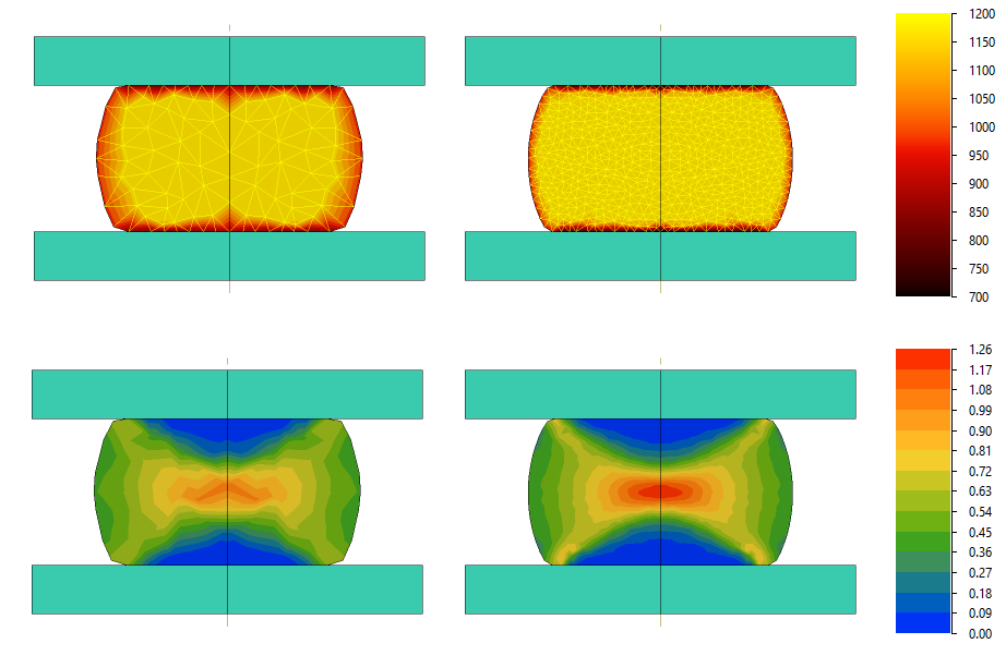
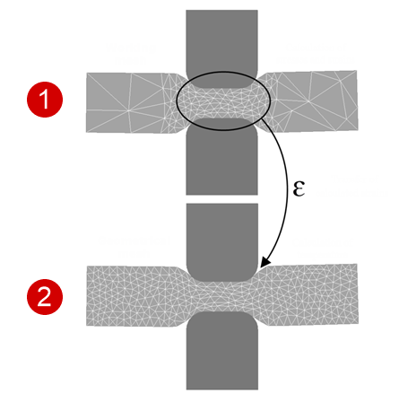
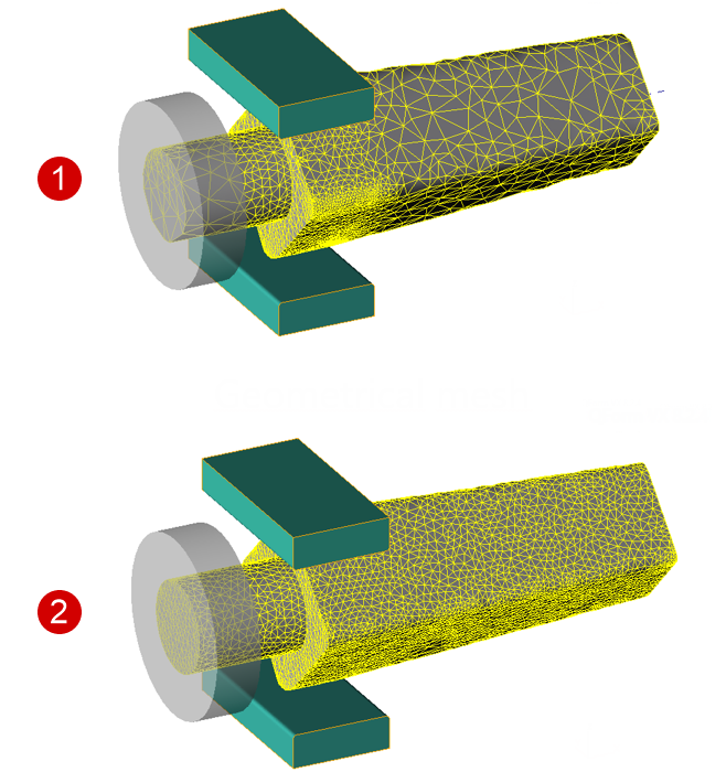
In metal forming process simulations, the main part of the computational time is spent on the calculation of stresses and displacements in the nodes of the finite element mesh of the deformed workpiece. Therefore, it is reasonable to minimize the number of nodes in the unloaded regions of the workpiece. On the other hand, the body shape and the accumulated strain field must be accurately preserved throughout the entire simulation, and the thermal problem must be solved with optimum accuracy throughout the entire volume of the workpiece, including outside the deformation zone. When using the dual mesh method in QForm UK, the first mesh, called the calculation mesh, is used to calculate the stress and accumulated strain fields. The calculation mesh is fine only in the deformation zone and coarse throughout the remaining volume. The second mesh, called the geometrical mesh, is used to preserve the shape of the deformed body and the accumulated plastic strain field transferred from the calculation mesh. In this setup, the thermal task is solved on the geometrical mesh. The geometrical mesh must be fine throughout the entire volume of the deformed body, and its density should match the density of the calculation mesh in the deformation zone. The figure below shows the principle of the dual mesh method implemented in QForm UK. Top: the calculation mesh with fine elements in the deformation zone and coarse elements throughout the remaining volume. Bottom: the geometrical mesh with fine elements throughout the entire volume.
The dual mesh method can be used effectively to speed up simulations of processes with a localized deformation zone - such as open die forging, ring rolling, longitudinal rolling, and rotary tube piercing - and to achieve a more accurate computation of temperature fields in any metal forming processes.
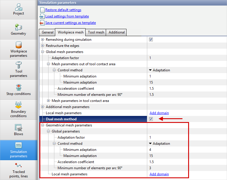
It is difficult to assess the advantages of the dual mesh method based on any single example. The increase in simulation speed depends on the type of process being simulated and on the finite element mesh parameters. In some cases, the speed can be improved by an order of magnitude, for example in rolling of a wide sheet. To use the dual mesh method, go to Workpiece mesh and enable Dual mesh method. A Geometrical mesh parameters block will then appear below:
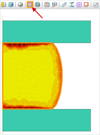
When viewing the simulation results, you can display either the calculation mesh or the geometrical mesh using the corresponding buttons on the toolbar:
|
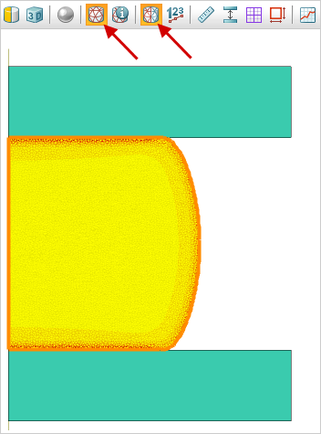
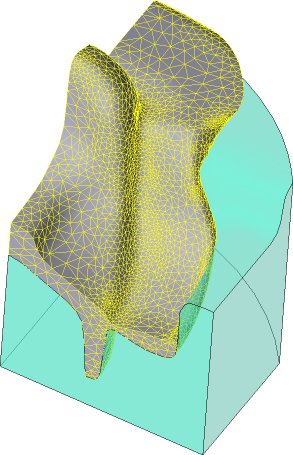
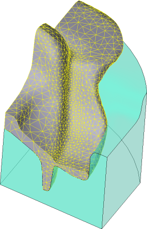
During the simulation in QForm UK, the workpiece mesh is automatically adapted to the mesh of the contacting tool. Once the Tool is no longer in contact with the Workpiece, the Mesh parameters out of tool contact area are applied to the released region of the workpiece, and the workpiece elements may begin to coarsen, which can distort the deformed region. To prevent this, you need to activate Prohibit increasing of element size option in Workpiece mesh section:
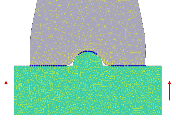
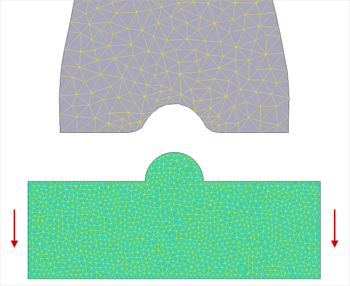
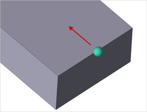
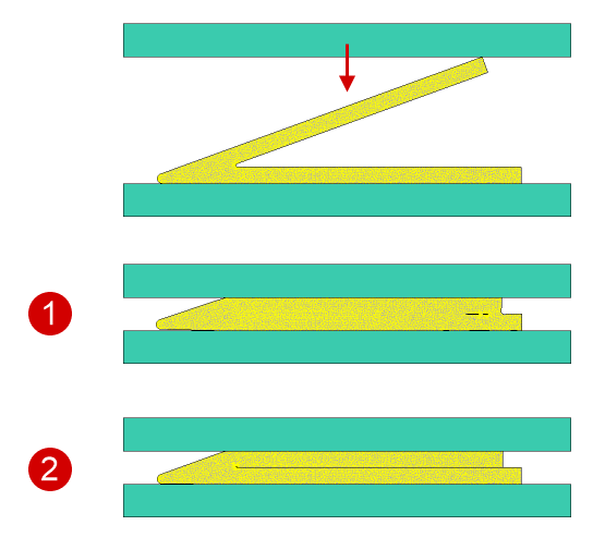
Let’s consider how the parameter works using a simple example. The tool with a spherical shape creates a groove on the workpiece:
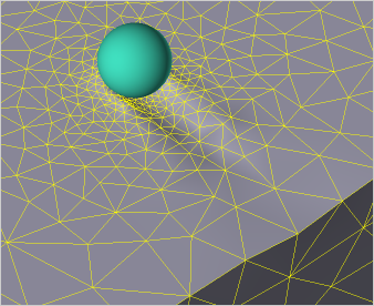
In the contact area with the spherical tool, the Workpiece mesh inherits the dense mesh parameters of the tool. When contact with the sphere is lost, the Mesh parameters out of tool contact area are applied to the previously deformed region of the workpiece, and the deformed geometry is distorted. The figures below show that the prohibit increasing of element size solves this problem:
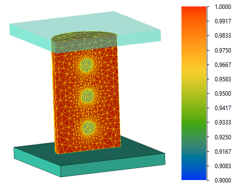
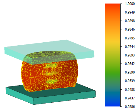
Another example where the Prohibit increasing of element size parameter can be useful is in evaluating the structure refinement of a forged ingot. The figures below show the simulation of upsetting a cylindrical ingot using a symmetry plane. At the start of the simulation, three local mesh-parameter regions were defined for the workpiece, each with a relative density of 0.9. For these same workpiece regions, a denser mesh was assigned using boxes. During the simulation with the prohibit increasing of element size, the mesh elements in these regions do not grow larger, which helps maintain the accuracy of the computed relative density fields without averaging:
|
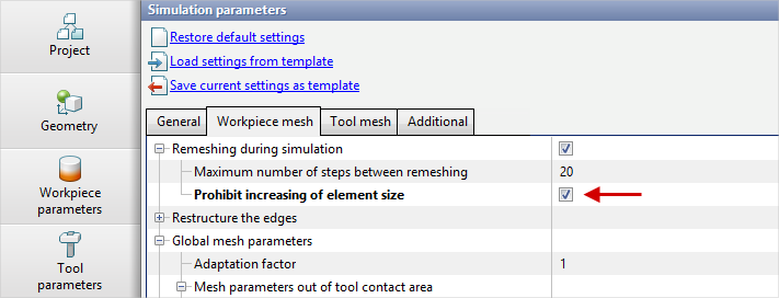
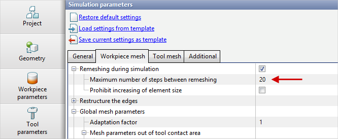
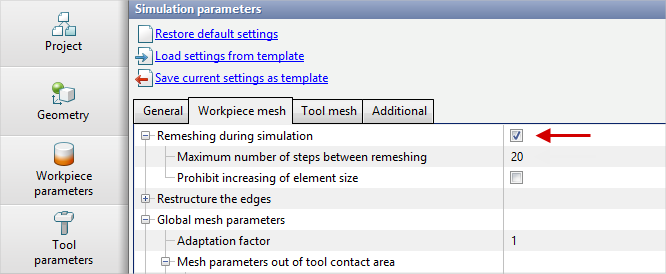
During the simulation, the workpiece mesh is automatically remeshed when certain conditions are met. If no remeshing conditions arise, the workpiece is remeshed, by default, no more than once every 20 calculation records:
In some cases, it is advisable to force remeshing at every record. To do this, set the parameter Maximum number of steps between remeshing to 1. For example, this ensures the workpiece mesh adapts in time to the approaching Tool mesh. In other cases - e.g., when the workpiece mesh deforms only slightly and does not need to adapt to the curvature of the deforming tool or to changes in its own surface curvature - it is recommended to disable remeshing altogether. Disabling remeshing in such cases can both speed up the simulation and improve the accuracy of the results. To disable it, clear the checkbox for Remeshing during simulation.
Disabling remeshing can also be useful, for example, when simulating spring compression up to the moment coil-to-coil contact occurs. |
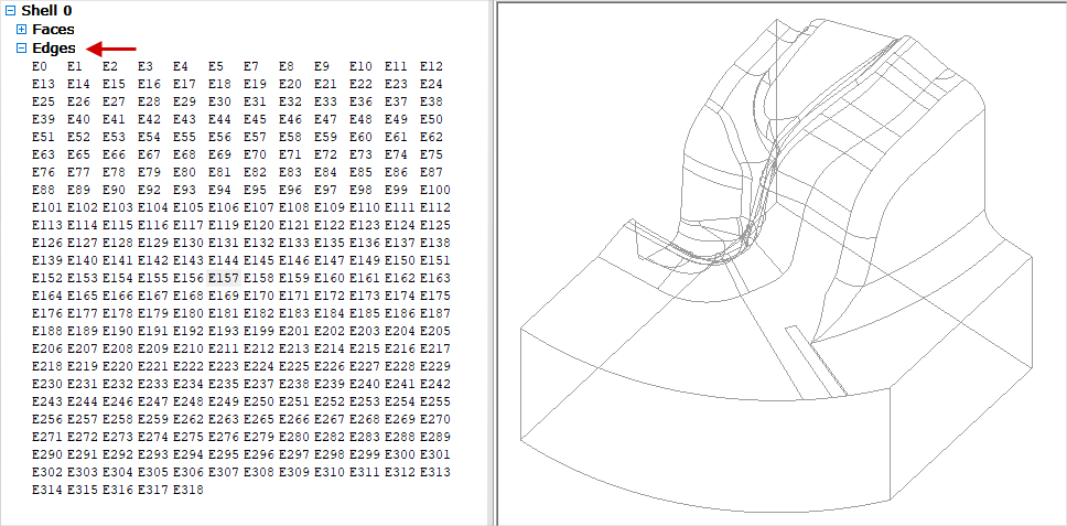
The original parametric geometry of the workpiece and tools, prepared in a CAD system, has edges that bound the surfaces.
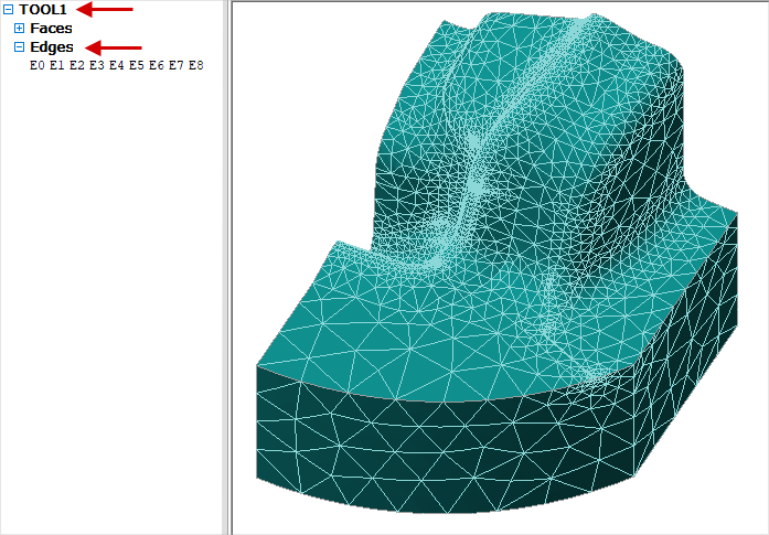
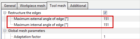
After surface mesh generation, the geometric object structure is preserved with the same number of surfaces and edges. After converting the generated surface mesh to a specific object type (Tool or Workpiece), the surface-mesh structure changes: some surfaces are merged, and consequently the number of edges decreases:
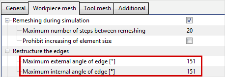
After the surface mesh is loaded into QForm UK and the simulation is started, a volume mesh is generated for all objects. By default, the Maximum external angle of edge and Maximum internal angle of edge parameters for the Workpiece and Tool meshes are set to 151°. The edge angle is the angle between the surfaces that the edge separates.
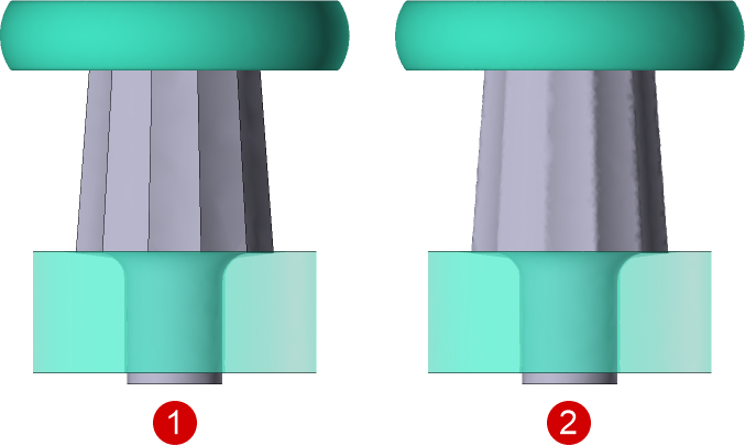
Depending on the specified maximum edge-angle values, some edges on the surface of the generated volume mesh may either be reconstructed or, conversely, removed. The larger the maximum edge angles, the more edges will be created on the workpiece or tool volume-mesh surface - and vice versa. Moreover, under certain conditions during deformation and remeshing, edges on the workpiece surface may appear or disappear.
As the example illustrates, for complex geometries with many curved regions it is difficult to predict the effect of changing these parameters. Therefore, it is recommended to modify the default values only when you understand the consequences. In some cases, improper changes to the maximum edge angles can lead to errors during volume-mesh generation.
|
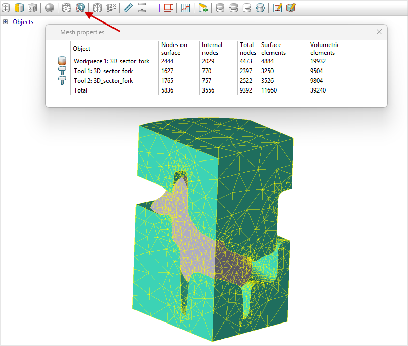
There are several ways in the program to assess the calculation mesh density, Adaptation values, and element sizes. To obtain the total number of volume and surface nodes and elements for all workpieces and tools, click the corresponding toolbar button:
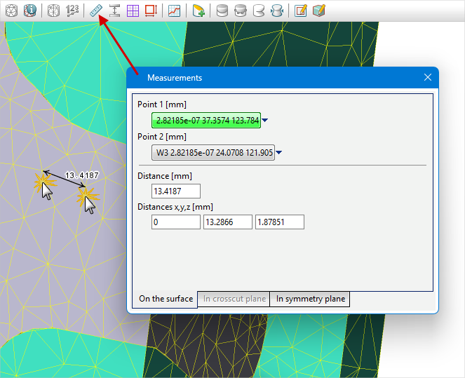
The computational “load” is usually judged by the values in the Total nodes column. When simulating an uncoupled task with rigid tools, it is recommended to evaluate the total number of nodes in the workpiece only. When simulating a coupled deformation task, the sum of nodes in the workpiece and the tools (for which the stress-strain state is computed) affects the simulation speed. Using the Measure tool, you can roughly estimate the size of an element of interest. In On the surface mode, specify the coordinates of two points: with Ctrl pressed, double-click to select two nodes of the element in sequence:
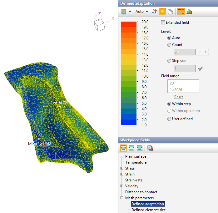
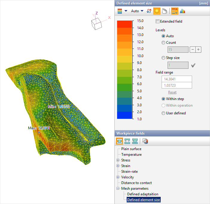
Additionally, in the list of computed fields for the workpiece or tool, under the Mesh parameters field block, two fields are available: Defined adaptation and Defined element size.
These fields are also available in the General fields list. Thus, you can display the distributions of Defined adaptation and Defined element size simultaneously for both the workpiece and the tool. |
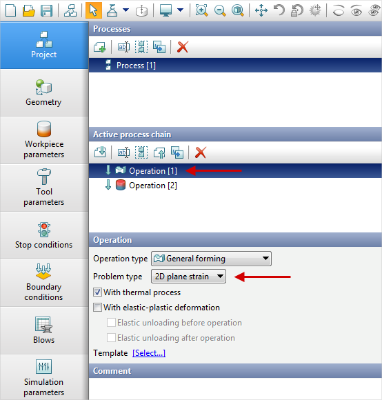
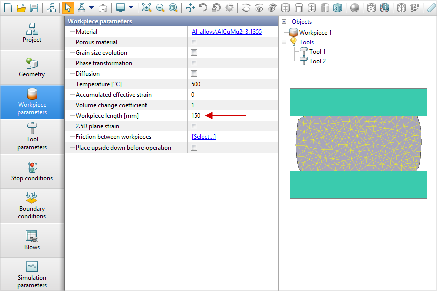
In a 2D plain strain task, you must specify the workpiece length in the workpiece parameters:
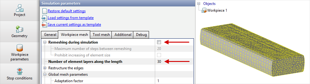
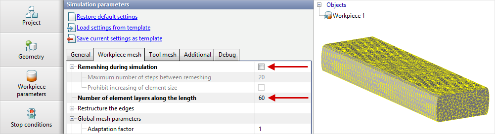
When running the 3D operation, you can create a regular 3D mesh from the inherited 2D workpiece mesh. To do this, in the 3D operation’s simulation parameters, under Workpiece mesh, disable Remeshing during simulation and specify the required number of element layers along the length:
|
|
Important |
Some inconsistent combinations of finite element mesh parameters may lead to unpredictable results. It is therefore recommended to change mesh parameters guided by common sense. |
|