One of the main purposes of using simulation in the development of technological processes is to determine the optimal processing parameters, that provide the minimum number of steps required to produce the part from the initial workpiece, also on the basis of predicting the occurrence of workpiece defects during processing. To identify the occurrence of workpiece defects in sheet metal forming, forming limit diagrams are widely used.
Forming limit diagrams are plotted on the coordinate plane with the minor principal strain in the sheet surface (εmin) along the x-axis and the major strain (εmax) along the y-axis. Strain hereinafter means true strain. Information about the existing types of strain can be found in the documentation section Displacements, strains and strain rates.
The region of positive εmin of the forming limit diagram corresponds to biaxial tension, while the negative one to uniaxial tension. In the case when the value of εmin is zero, a plane strain state is realized. The forming limit curve is plotted on the coordinate plane, which represents the critical values εmax as a function of εmin at which a crack will form on the workpiece. Thus, there are points of all possible combinations of εmin and εmax above the forming limit curve which correspond to the fractured workpiece (the failure zone of the forming limit diagram). Forming limit curves were first introduced in the works [1, 2]. The forming limit curve is unique for each sheet material and depends, among other factors, on its thickness. There are different experimental, empirical, semi-empirical and theoretical methods to determine the forming limit curve [3]. Theoretical, empirical, and semi-empirical methods either require a small number of simple tests or none at all, but they do not always provide reliable results. The most accurate are experimental methods, but they are typically associated with the need to conduct a large number of experiments using specialized equipment and tooling. Many different experimental methods have now been proposed to determine forming limit curves [3]. Among these, ISO 12004 has been developed, the second part of which is devoted to determination of the forming limit curve for sheet metals with thickness from 0.3 mm to 4 mm (for steel materials the standard recommends limiting the maximum thickness to 2.5 mm) at room temperature through tests with constant values of εmax/εmin during loading.
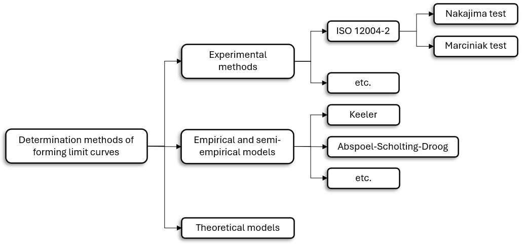
The model uses empirical equations derived by analysing experimental data obtained mainly for low-carbon steels. These equations allow us to determine the forming limit curve (FLC) of material by the initial sheet thickness (t) and the value of its strain hardening exponent (n), which is taken as the exponent of the Ludwick-Hollomon equation approximating the hardening curve. In 1975, Keeler and Brazier first proposed using an empirical equation to determine the value of the limiting strain under plane strain conditions (ε10) [4]:
It was assumed that the shape of the forming limit curve remains unchanged, and it is enough to shift the curve along the vertical axis to obtain one that corresponds to a other value of ε10. Subsequently, the given equation was refined and supplemented in various works. Currently, the Keeler model, in its original or modified form, is one of the most widely used models for predicting the forming limit curve of a material due to its simplicity and the absence of the need for complicated experiments.
|
||||
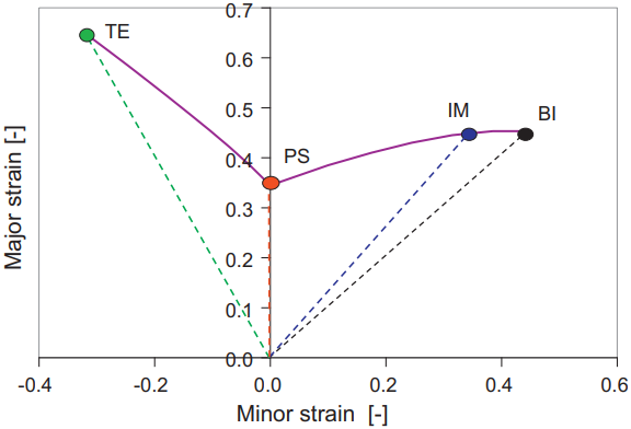
Abspoel, Scholting and Droog have analysed the relationship between the forming limit curve and other mechanical properties of the material in [5]. Based on the obtained data, equations were proposed for calculating the limiting strains at specific points on the curve. So the authors identified four points on the forming limit curve by reviewing previous work in this area:
where TE - the limit state point for loading along the trajectory that corresponds to uniaxial tension; PS - the limit state point for loading along the trajectory that corresponds to plane strain; IM - the limit state point for loading along the trajectory that corresponds to intermediate biaxial stretch, at which the strain ratio is 0.75; BI - the limit state point for loading along the trajectory that corresponds to equi-biaxial stretch. The study was performed subsequently to determine the relationship between the experimentally obtained values of the forming limit curve at these points and the various mechanical properties of materials that were determined by uniaxial tension of flat specimens for a wide range of modern steels. As a result, relationships have been established that are suitable for nearly all the examined materials and allow to determine the limiting strain values at these points using the following parameters: •A80 - total elongation of a flat specimen, the longitudinal axis of which coincides with the direction for which the forming limit curve is calculated, determined according to ISO 6892-1; •A80min - the smallest among the values of parameter A80 that are determined for three types of specimens: with the longitudinal axis coinciding with the rolling direction, perpendicular to it and located at an angle of 45°; •r - plastic anisotropy coefficient,which is defined according to ISO 10113 for the flat specimen whose longitudinal axis coincides with the direction for which the forming limit curve is determined; •t - initial sheet thickness. The forming limit curve is obtained by connecting these points. The resulting equations were tested on fifty different grades of steel.
|
||||
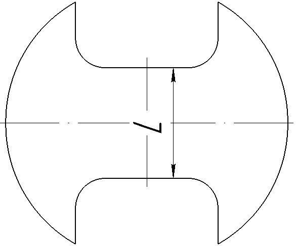
The sample used in tests according to this standard has a shape resembling a dog bone (in some cases, the use of flat specimens of various widths or specimens differing from the one shown below by having side notches shaped as arcs of a circle is also permitted):
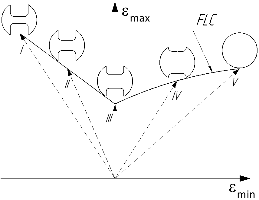
The width L of the central section of the specimens used in various tests varies. This allows to change the value of εmax/εmin and to obtain different points of the forming limit curve (tests are conducted until a split appears on the sample). So, if the jumper is narrow enough, uniaxial tension is realised in the sample, and if the sample without side notches (in the form of a disc) is used, equi-biaxial stretch is realised. Varying the width of the jumper between these two extreme values allows to achieve different intermediate states and points of the forming limit curve. The minimum required number of different loading paths according to the standard is 5. It is recommended that they be evenly distributed along the forming limit curve. Then, by connecting the obtained points, the forming limit curve of the investigated material is obtained:
where I, II, III, IV, V - trajectories of strain state evolution in samples during tests with different ratio values εmax/εmin, at the end of which the samples corresponding to them are shown schematically; I - the trajectory of uniaxial tension with εmax/εmin=(-Rm- 1)/Rm (here Rm - average value of the Lankford coefficient); III - the trajectory that corresponds to the plane strain state with εmin=0; V - the trajectory that corresponds to the equi-biaxial stretch with εmax/εmin= 1; II, IV - trajectories that are intermediate between the trajectories described above; FLC - forming limit curve. For accurate measurement of strain values, a special grid with elements of specified sizes is drawn on the sample, or the DIC method is applied. To determine the forming limit curve of anisotropic material, the samples that are cut from the sheet should be oriented so that their longitudinal axis coincides with the direction of the sheet along which εmax value is minimal. So this direction is generally perpendicular to the rolling direction (RD) for steel, and parallel for aluminum alloys:
Tests can be performed according to the standard using either the Nakajima method or the Marciniak method. This requires the application of different methods to minimise the impact of friction between the sample and the tools in order to accurately determine the forming limit curve. In tests by the Nakazima method, sample 1, the flange section of which is rigidly clamped between die 2 and blank holder 3, is formed to failure by the hemispherical punch 4:
The lubricant used in tests by this method must ensure that the sample fractures at a distance of less than 15% of the punch diameter from its apex. Only in this case the test results are considered valid. Thus, the standard suggests the use of different lubrication systems that depends on the investigated material. In the Marciniak tests, sample 1 with a flange rigidly clamped between die 2 and blank holder 3 is formed to failure by a cylindrical punch 4 with a flat bottom:
In this case, to minimise the impact of friction on failure and the occurrence of a crack in the central part of the sample, the additional blank 5 from a softer material with a hole in the centre is placed between the sample and the punch. For detailed information on the methodology for processing test results, equipment requirements, and other details, it is recommended to refer to the standard. |
||||||
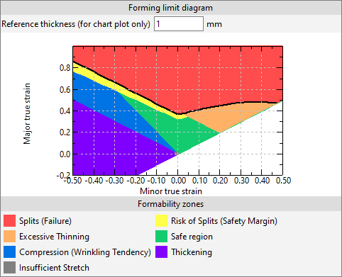
In addition to plotting the forming limit curve above which the failure zone is located, other formability zones are also marked on the coordinate plane of the forming limit diagram. As a result, it looks like this:
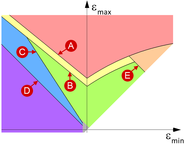
Lines used: |
|
|
- forming limit curve; |
|
- the curve obtained by shifting the forming limit curve on a specified value along the ordinate axis; |
|
- the straight line εmax = (-Rm- 1)/Rmεmin (here Rm - average value of the Lankford coefficient); |
|
- the straight line εmax = -εmin; |
|
- the straight line εmax = -εmin + εET (here ε ET - maximum allowable thinning). |
Regions of the forming limit diagram (formability zones): |
|
|
- zone of splits (failure); |
|
- zone of risk of splits; |
|
- zone of excessive thinning; |
|
- safe region; |
|
- zone of compression (wrinkling tendency); |
|
- thickening zone; |
|
- zone of insufficient stretch. |
|
Important |
The forming limit diagrams in QForm UK should generally be used for the analysis of cold sheet metal forming operations with a plane stress state in the workpiece and a constant ratio of εmax/εmin. |
|
The forming limit diagram in QForm UK is calculated using the corresponding standard post-processing subroutine. Information about the available standard subroutines and their usage can be found in the documentation section Subroutines.
|
Important |
The calculation subroutine Forming limit diagram (FLD) is available in simulations with a hexahedral mesh of the workpiece or with a tetrahedral mesh if the option of its remeshing during simulation is disabled. In the latter case, the output fields of the subroutine are calculated only for the elements of the surface layer of the mesh. |
|
The components of the strain state tensor in elements of the workpiece mesh are determined at each calculation step in during the simulation. The output fields of the Forming limit diagram (FLD) subroutine (hereinafter referred to as the subroutine) are calculated on their basis. The subroutine has three output fields:
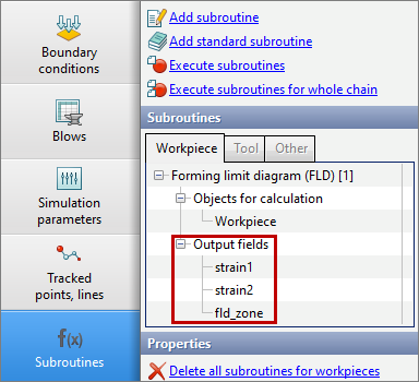
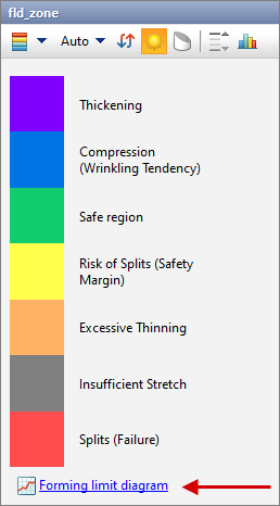
The first field is strain1 that displays values of εmax, the second one is strain2 that displays values of εmin, and the last one is fld_zone that colors the workpiece mesh elements in the color of formability zones corresponding to εmin and εmax values in them. If the fld_zone field is selected, the Forming limit diagram button appears below the results scale. Clicking on it displays the window of the same name which contains the forming limit diagram for the active calculation step:
|
|
|
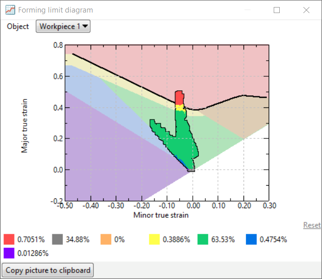
The points on the diagram are plotted by values of εmin and εmax in the workpiece mesh elements. If the mouse cursor hovers over any workpiece mesh element, the corresponding point on the forming limit diagram will be highlighted with a black frame.
In the lower part of the Forming limit diagram window, percentage values show which portion of the workpiece material volume located in each formability zone of the corresponding colour.
The section of the limit deformation diagram that interests you can be enlarged by selecting it with a frame that appears when you hold down the left mouse button. After that, the Reset button, which was initially inactive and located in the lower right corner of the Forming limit diagram window, will become available. When you click it, the zoom will be cancelled and the diagram will return to its original view.
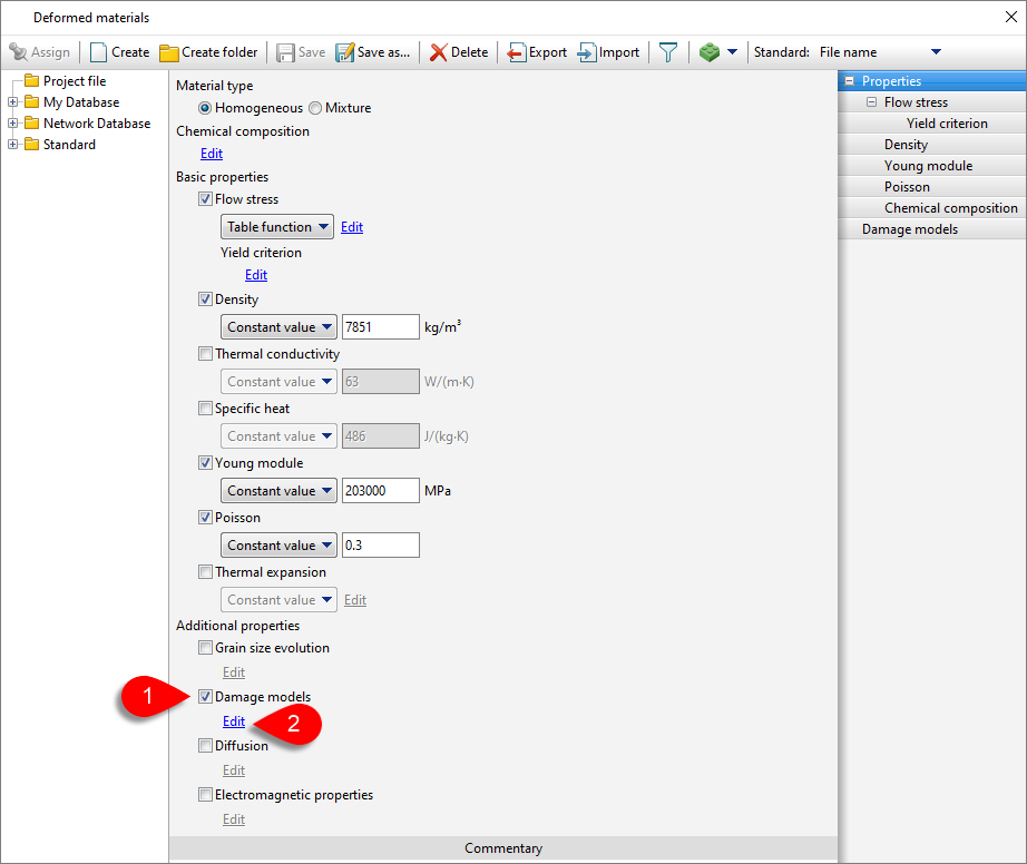
For the correct calculation of the subroutine it is necessary to activate Damage models in section Additional properties of the database Deformed materials for the workpiece material used in the simulation and then click on Edit below this property:
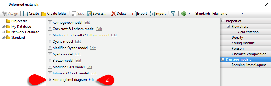
From the list of available models, select the Forming limit diagram model and then click Edit next to it.
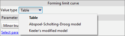
In the displayed window, it is necessary to define the forming limit curve. Three methods of assignment are now available in QForm UK:
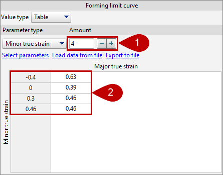
When the Table method is used, the forming limit curve is obtained by connecting the points, whose coordinates are determined by the values specified in the table cells, using a polyline of linear segments. In this case, it is necessary to specify the number of input points for the forming limit curve (1) and their values of εmin and εmax (2):
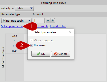
Using the Load data from file and Export to file buttons, you can load the points of forming limit curve from a *.csv, *.xls or *.xlsx file, or export them to these files. If it is necessary, you can activate the thickness of the initial sheet material (2) as the second argument of the table function on which the εmax value of the points of the forming limit curve depends by clicking the Select parameters button (1):
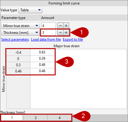
In this case it will also be necessary to specify the number of thickness values for which the forming limit curve is defined (1), their values (2) and, for each of them, the value of εmax at the selected values of εmin (3):
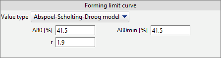
When the Abspoel-Scholting-Droogmodel is used to set the forming limit curve, values of parameters A80, A80min and r must be set (parameter descriptions are given earlier in the section with information about this model):
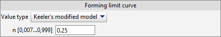
When the Keeler's modified model is used for setting the forming limit curve, the value of the strain hardening exponent of the material n must be set:
The thickness value of the initial sheet, that is used in Abspoel-Scholting-Droog model and Keeler's modified model to determine the forming limit curve of the material, is taken equal to the workpiece thickness that is used in the simulation.
The parameters of the formability zones are also set in the window for specifying the forming limit diagram:
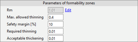
For the most part, the value of these parameters is determined by the requirements for the resulting product. The value of the parameter Safety margin [%] sets the amount of displacement of the forming limit curve to determine the position of the zone Risk of splits and, as a rule, is taken equal to 10%.
|
Important |
The major and minor strains which define the points on the forming limit curve, as well as the parameters of the formability zones, are specified in terms of true strain values. |
|
Below the parameters of formability zones in this window, the coordinate plane of the forming limit diagram is displayed according to the entered data. When Abspoel-Scholting-Droog model or Keeler's modified model is used, it is required to specify in the Reference Thicknessfield the initial sheet thickness that will be used only in this section to visualise the position of the forming limit curve on the diagram:
|
Important |
To determine the position of the failure zone on the forming limit diagram, ifεmin or the initial thickness of the workpiece is outside the range for which the forming limit curve is defined in the material model, the value of εmax is not extrapolated, but is taken equal to its value for ε min or initial thickness from the defined range, which are closest to the specified values of the parameters. |
|
1.Keeler, S. P.: Plastic instability and fracture in sheet stretched over rigid punches, Thesis, Massachusetts Institute of Technology, Boston, MA 1961. 2.Goodwin, G. M.: Application of strain analysis to sheet metal forming problems in the press shop, Society of Automotive Engineers (1968), No. 680093, 380-387. 3.Formability of Metallic Materials: plastic anisotropy, formability testing, forming limits / D. Banabic... Ed. by D. Banabic - Berlin ; Heidelberg ; New York; Barcelona; Hong Kong; London; Milan; Paris ; Singapore ; Tokyo: Springer, 2000. 4.D. Banabic (ed.), Multiscale Modeling in Sheet Metal Forming, ESAFORM Bookseries on Metal Forming, DOI 10.1007/978-3-319-44070-5, 2016. 5.M. Abspoel et al. A new method for predicting Forming Limit Curves from mechanical properties / Journal of Materials Processing Technology 213 (2013) 759-769 |