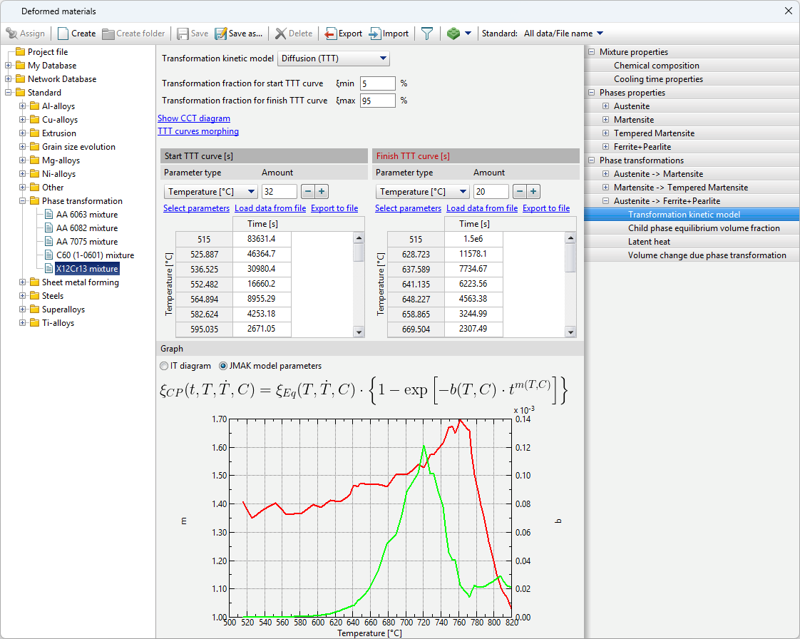
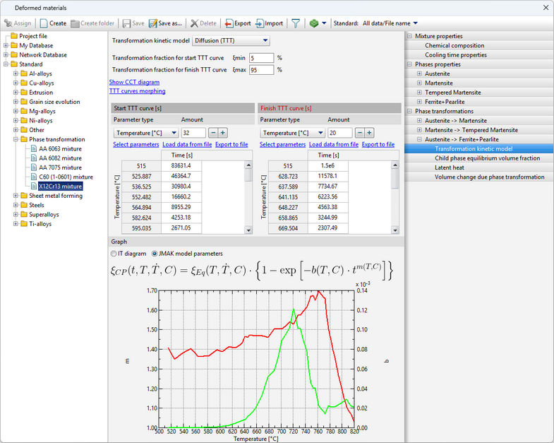
The JMAK (Johnson-Mehl-Avrami-Kolmogorov) model is used for calculation, the parameters of which are given by the TTT-diagram

The diagram represents curves corresponding to the beginning of the transformation (volume fraction of the child phase ξmin), the selected value of the transformation fraction (the Show the curve for the transformation fraction option) and its completion (volume fraction of the child phase ξmax). The chart shows how long it takes for the child phase share to increase from ξmin to ξmax at a given temperature. Since the typical values given in the reference literature for ξmin and ξmax are 1 and 99% or 5 and 95%, then the total phase transformation time at a given temperature can be estimated from the diagram.

In addition, it is possible to display the kinetic curve for a given temperature on the graph by clicking on theShow the kinetic curve option.

The labels of these curves are displayed when you hover the cursor over them.

When specifying data, attention should be paid to the following:

•For phase fractions on the curves, the following relation must be satisfied: 0% < ξmin < ξmax < 100%.

•TTT curves are specified by tables that may have different numbers of rows, however, the maximum and minimum temperatures for both curves must be the same. Also, the onset time and duration (distance between curves) of the transformation must be greater than 0 for all temperatures (i.e., the curves must not overlap). If the specified limits are not met, a corresponding error message appears.

•TTT curves are not extrapolated by temperature.

•In modeling of steel quenching processes, this transformation model is usually used to describe the kinetics of transformation of austenite into ferrite, pearlite and bainite.

For different materials, TTT diagrams can be found in the reference literature:

1.Popova L.E., Popov A.A. Diagrams of austenite transformation in steels and beta solution in titanium alloys: Thermist's Handbook. 3rd ed., rev. and supplement. M.: Metallurgy, 1991.

2.Atlas of Time-Temperature Diagrams for Irons and Steels / Ed. by G.F. Vander Voort. Vander Voort. ASM International, 1991.

3.Atlas zur warmebehandlung der stahle / F. Wever, A. Rose, W. Peter, W. Strassburg, L. Rademacher. Dusseldorf: Verlag Stahleisen M.B.H, 1961.

The tab Graph displays selection buttons are present: Isothermal Transformation diagram and JMAK model parameters. The isothermal transformation (IT) diagram is displayed by default. After switching to JMAK model parametersthe graphs of the m and b coefficients of the equations will be displayed.

If this option is selected, the formula from which these coefficients m and b are calculated will also be displayed above the graph with coefficients. When you hover the cursor over curves, their labels are displayed; when you hover the cursor over variables in the equation, their names are displayed.

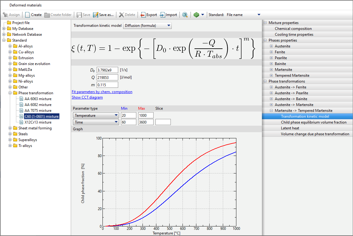
The JMAK model is used for calculation, the transformation kinetics is described by the formula

,

where D0 is the pre-exponential constant, Q is the activation energy, R is the universal gas constant, Tabs - absolute tempering temperature.

The model is recommended to be used for modeling tempering processes of steels, i.e. for the phase transformation of martensite into tempered martensite.

Parameter values D0, Q and m for some carbonaceous tool steels can be adopted from the work Zhang Z., Delagnes D., Bernhart G. Microstructure evolution of hot-work tool steels during tempering and definition of a kinetic law based on hardness measurements // Materials Science and Engineering A. Vol. 380. 2004. P. 222-230.

Similarly as with other diagrams in QForm UK databases, in this graph you can change the interval of displayed values and write any parameter value in the Slice cell to draw a black curve for the specified parameter value. It is also possible to change the horizontal scale on the graph by clicking on the expandable list Parameter Type (1).

When you click on Fit parameters by chemical composition (2), an additional window will appear where you can select which properties to copy to a given phase transformation. These properties are obtained by computation using a choice model:

1.R.A. Grange, C.R.. Hribal, L.F. Porter Hardness of tempered martensite in carbon and low-alloy steels // Metallurgical transactions A, Vol. 8A (1977), p. 1775-1785

2.Monideepa Mukherjee, Chaitali Dutta, Arunansu Haldar Prediction of hardness of the tempered martensitic rim of TMT rebars// Materials Science and Engineering A, Vol. 543 (2012), p. 35-43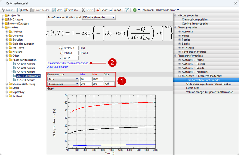

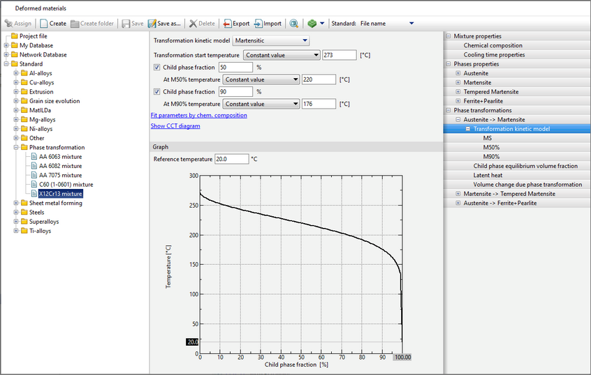
The Koistinen-Marburger model, described by the formula, is used to calculate diffusionless phase transformations, such as austenite to martensite during steel quenching:

,

where ξγ - volume fraction of residual austenite; MS - temperature of the beginning of martensitic transformation. This formula is valid for carbon steels when MS> T > -80°C.

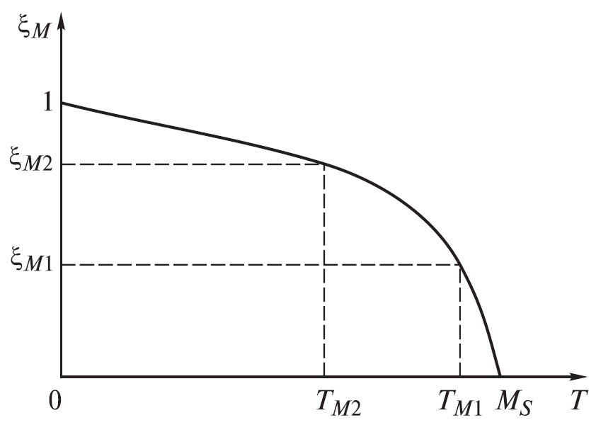
The Koistinen-Marburger model can be written in a more general form:

,

the parameters Ψ1and Ψ2 can be determined from one or two points of the experimental martensitic transformation curve.

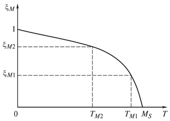
•If only the temperatureMS is set, then

Ψ1= 0,011;Ψ2= -0,011MS.

•If temperatures are set MS and TM1, and corresponding to temperature TM1 martensite fraction ξM1, then

•If two points on the experimental curve are known, the Lee – Van Tyne martensitic transformation model can be used:

,

where

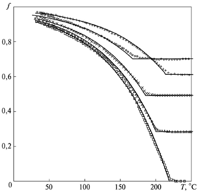
At the same time, the preceding course of other phase transformations practically does not affect the kinetics of martensitic transformation, but decreases its onset temperature.

To take this feature into account in the Koistinen-Marburger and Lee – Van Tyne models, the corrected value of temperatureT'should be substituted instead of temperatureT:

,

whereT1is a fictitious temperature determined from the current concentration of all other phases (except for the parent and child phases for a given phase transformation).

For the Koistinen-Marburger model it is calculated by the formula:

For the Lee – Van Tyne model is calculated using the formula:

Here

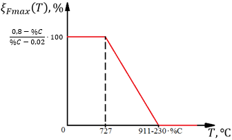
takes into account the presence of other phase transformations (CP - child phase; MP - mother phase) and possible thermodynamic constraints on the equilibrium volume fraction of the child phase. At that, if T > T1, the transformation does not proceed.

In QForm UK the Koistinen-Marburger and Lee - Van Tyne models are used in differential form:

The model can be used to describe the kinetics of both diffusive and martensitic transformations.

The model is described in Leblonde J.B., Devaux J. A new kinetic model for anisothermal metallurgical transformations in steels including effect of austenite grain size // Acta metal. 1984. Vol. 32 (1). P. 137-146.

The user needs to set table functions τ=f(T)>0 and

In the case of hardening steels, Leblonde J.B. and Devaux J. propose to set values ​​ for all transformations except the transformation of austenite into bainite.

Function ξmax=f(T) represents the child phase equilibrium volume fraction.

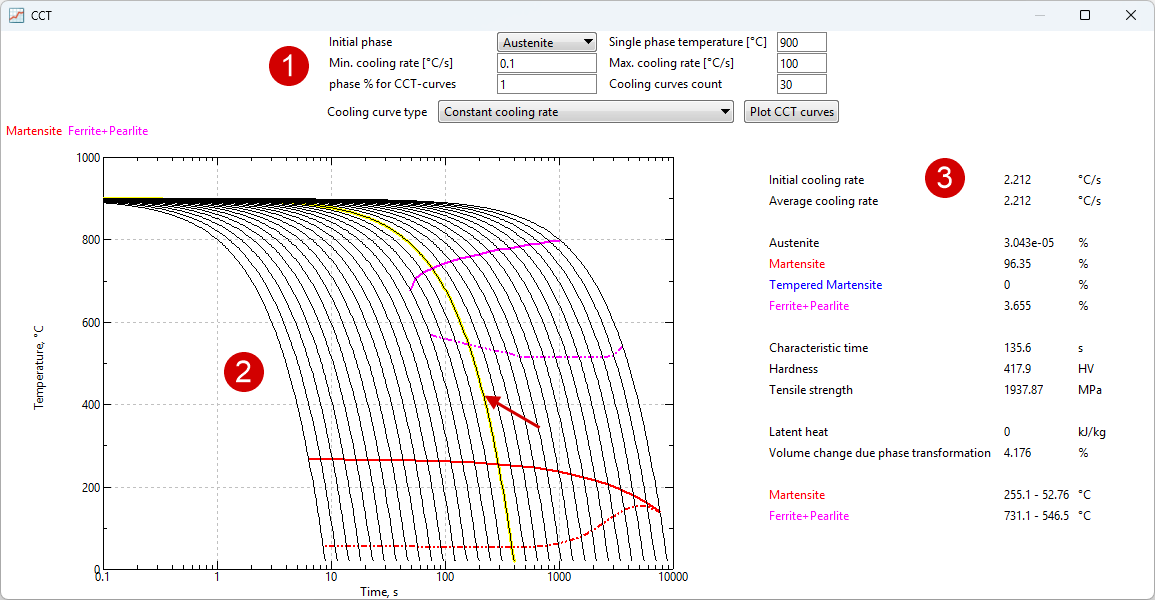
After creating the properties of the kinetics of all phase transformations required for a given material, it is possible to display the CCT (continuous cooling transformation) diagram. It is calculated within the program on the basis of specified models of phase transformation kinetics. Such a feature is designed to allow the user to evaluate the correctness of the given properties of phase transformations and compare the CCT-diagram with a reference or experimental one.

To display the CCT diagram window, you must click Show CCT diagram in the Phase transformations tab. It can also be displayed by clicking on a similar label in the Transformation model tab.

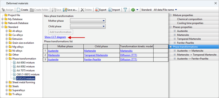
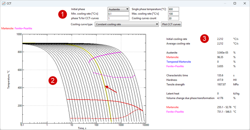
The window CCTcan be roughly divided into three zones:

1.Diagram display settings.

2.CCT diagram. If you move the cursor over a cooling curve in zone 3, information about it is displayed.

3.Predicted properties after cooling at a given (highlighted curve) rate.