Flow stress is the effective stress acting at uniaxial tension along sample axis at the stage of uniform deformation (up to necking).
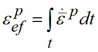
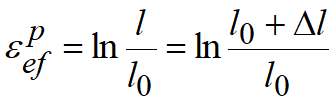
During plastic deformation the flow stress usually increases. In QForm UK a strain hardening hypothesis is implemented, according to which the hardening quantity is determined with the effective plastic strain
The flow stress dependency on effective strain, strain rate and temperature can be described as follows:
![]()
is considered as description of constitutive behavior of material independently on the stress state mechanism, in other words this is a characteristic of material flow stress behavior. A single curve concept provides the possibility to use the compression and torsion tests for determination of material rheological properties.
Material flow stress is determinative of the deforming force obtained as a result of simulation.
Temperature increase at plastic deformation causes the flow stress reduction. For the majority of materials at cold deformation the increase of flow stress with increase of effective strain and strain rate is inherent. This effect is called strain hardening and strain-rate hardening, respectively. The graph of dependence of flow stress on cumulative (effective) strain at constant temperature and constant strain rate
is called the hardening curve. For some metals at elevated temperatures and small strain rate a phenomenon of softening occurs that is related to dynamic recrystallization. |


Flow stress of metal at simulation in QForm UK is chosen from the materials database. If chosen material is absent in database, its properties are determined experimentally and then stored in the database. It is recommended to perform the experimental research on determination of material properties even, if the material is available in the database. The database in QForm UK is composed on the basis of literary sources analysis, however, the results of different authors' experiments often differ from each other even for the same material. In order to determine the flow stress (hardening curves) different methods are used. The most common are tensile test, compression test, and torsion test. It is recommended to perform processing of experimental results with the inverse method. During tests it is required to maintain constant strain rate (not to be confused with testing machine grippers conveying speed) and sample temperature.
|

Flow stress depends on cumulative deformation, strain rate and temperature. In order to obtain exact results the tests on flow stress determination are carried out at constant values of parameters. However, it is unreachable in practice. However, it is unreachable in practice. The finite result is influenced by the deviations of testing conditions from simple stress states (uniaxial tension, uniaxial compression, uniaxial shear), which are related to influence of friction and inhomogeneity of strain and strain rate, heat generation in the course of plastic deformation. High accuracy of stress-strain state evaluation by means of finite element method permits using of simulation to specify calculation results. Traditionally the FE method is used for the prediction of metal flow and determination of strain energy and stress energy using the material rheological properties determined from testing as input data. Conversely, in the inverse method the FEM simulation is used for determination of material rheological properties by means of iterative approximation to experimental data on loads and specimen geometry.
For determination of rheological model parameters by inverse method it is necessary to pre-set the mathematical relation describing the model and determine the variable parameters. Then by varying, these parameters will achieve coincidence of test and simulation results. For example, if we use Hensel-Spittel formula as a material model
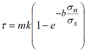
then these parameters are the coefficients A1,m1,m2,m3,m4. As far as it is impossible to eliminate the friction impact on experiments completely, then the friction factor m and coefficient b in Levanov's friction law should be considered as additional variable parameters
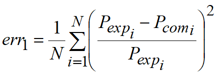
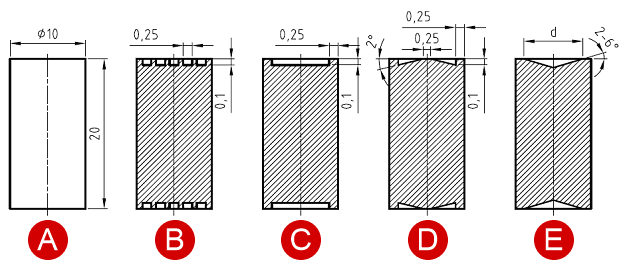
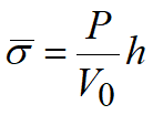
Then it is necessary to carry out the experiments by means of compressing the cylindrical specimen and determine the load graph ( the dependence of strain energy on strain path P=f(S)) and the specimen geometry ( the diameters of characteristic cross-sections). After selecting the initial approximation of variable parameters (e.g. from technical literature) the experiment simulation with FE method is carried out, for example, by means of QForm UK. Due to results of mathematical simulation the loading graph and the specimen geometry is determined. Error of calculation of strain energy can be determined, for example [see. Hyunjoong Cho (2007)], as a root-mean-square deviation of strain energy according to the experiment results Pexp and calculation of Pcom for several points of the loading graph.
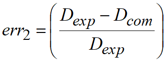
The error for prediction of geometric shape can be determined by comparison of maximum diameters (barrel diameter) in the experiment and in calculations
Cumulative error is determined as a sum of
If the simulation error exceeds the preset accuracy, a new set of variable parameters is generated and the simulations are repeated. The generation of new variable parameters is carried out either by means of gradient methods [Cho, 2007], or by means of downhill simplex method [Yun (2011)]. Simulation cycle is completed if the simulation error does not exceed the preset value and the variable parameters increments at the next step are negligible. Cho (2007) recommends selecting the parameters in sequence - first, selecting the parameters of the hardening curve due to strain energy graph, and then selecting the parameters of friction law due to workpiece shape. |