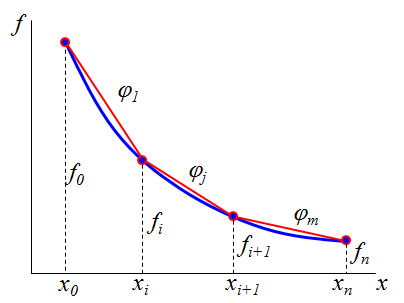
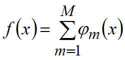
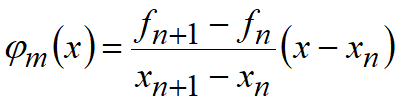
FEM basic idea is based on the principle that any continuous function f can be approximated with a set of more simple functions jm, (m=1…M, M - number of domains), any of which is defined at one domain. For example, at piecewise linear approximation a linear function of one variablef(x) the domain of a function is divided into certain number of subdomains, and at every such subdomain the real function is substituted with a straight line jm(x) passing through the boundary points. The coefficients determining these lines equations depends on the value of a function at subdomain boundaries. Thus, a continuous function is substituted with a set of values at separate points, and function behaviour between the points is defined approximately. The increase of subdomains number leads to the increase of approximation accuracy.
|
|
In plasticity problems the unknowns are the velocities of a large (but limited) number of points. These velocities are calculated by finding a solution for a set of algebraic equations composed automatically by a specific algorithm. The coefficients in the obtained system depend on the material properties, material points coordinates, loading history, and boundary conditions.
In simplified form the finite element method is the method for solving problems of mathematical physics. It is based on the representation of analysed object as a set of small domains (finite elements - FE). In every domain the sought-for function is approximated with low-degree polynomials.
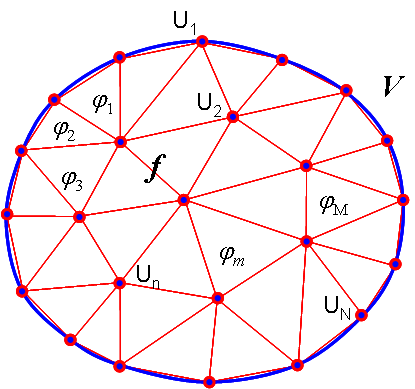
In general form the basic principles used for solution of problems on definition of function f which distribution in the domain V is undefined with finite element method can be formulated as follows: 1.The domain V is divided into simple subdomains known as finite elements. It is considered that the finite elements contact with each other in a limited number of points called finite element nodes.
2.The unknowns to be defined are the values of function in finite element nodes Un (n=1…N - total number of nodes). 3.The unknown function f is approximated with a collection of low-degree polynomials jm, (m=1…M, where M is the number of finite elements) possessing the following properties: 4.The method implements the variational methods for formulation of a set of governing equations: a problem of finding the values of unknown function in FE nodes, which give the best approximation to sought-for function true distribution, is set. The problem is solved by means of minimization of certain functional related to physics of the problem. 5. For every element the set of differential equations defining the object behaviour is transposed to a form:
called the element equations. Here [k(e)] - element stiffness matrix that depends on physical properties of continuum and element nodes coordinates, {u(e)} - column matrix of unknown values of function in element nodes, {P(e)} - column matrix of influence on finite element nodes by other finite elements and external effects. 6.All element equations can be assembled into a global system of equations - a system of linear algebraic equations with global vector of the unknowns in the nodes:
where [K] - global stiffness matrix defined due to a simple algorithm at known values of every element stiffness matrix components, {U} - vector of global unknowns, {R} - global right hand vector. 7.By solving the global system of equations are obtain the values for nodal unknowns Un, and then by means of polynomials jm the unknown function distribution over the entire domain is found. In a one-dimensional case the finite elements represent the small linear elements, in a two-dimensional case - small areas, in three--dimensional case - small volumes. In the simplest case for approximation of a function in finite element it is done by the first-order polynomials (linear functions). Such an elements are called linear. More accurate approximation can be achieved by using second order polynomials. Such an element is called quadratic. Coefficients of polynomials approximating the distribution of unknown function inside the element are uniquely determined with a function value in nodes and element dimensions. |
Finite element method procedure consists of the following sequence of steps: Pre-processor stage (data preparation) 1.Initial data analysis and choice of analytical model. 2.Assignment of element geometric form and dimensions in compliance with chosen the analytical model. 3.Definition of physical properties of continuum. 4.Selection of types of used finite elements. 5.Object discretization into finite elements. 6.Determination of boundary conditions. Determination of boundary conditions. 7.Determination of components of stiffness global matrix [K]and load global vector{R} as related to finite elements parameters and known external effects. 8.Rearranging of equation system according to boundary conditions. 9.Solving the equation system{R}=[K]{U} for unknown nodal variables vector. Post-processor stage (solution analysis) 10. Calculation of output parameters (e.g. strains, strain rates, stresses, forces, deformation work...), stipulated with problem formulation, due to derived values of unknown nodal variables. The sequence listed is characteristic for a linear problems solution. If the problem has essential nonlinearities (e.g. the presence of contacts is geometric non-linearity, plasticity is physical non-linearity), then the solution is carried out in several steps, for every one of which an iterative solution is obtained. In program QForm UK the processor stage is carried out fully automatically, and in the pre-processor and post-processor stages the user's work is automated to the fullest extent. |